VM0048: Baseline Emissions

Author

Seamus Murphy

Published

January 4, 2025

Abstract

A workflow for deriving activity data and emissions baseline compliant with Verra’s VMD0055 (V1.1) module and the VM0048 (V1.0) consolidated methodology.

Keywords

Jurisdictional REDD+, VCS, Carbon verification

1. Introduction

This workflow establishes baseline emissions estimates through systematic processing of satellite remote sensing data using cloud-based Earth Engine catalog and python API functions. The methodology integrates Analysis Ready Data (ARD) products with standardized atmospheric correction and quality assessment protocols to support jurisdictional REDD+ baseline development.

Study Area

The analysis focuses on a jurisdictional study area within the Upper Guinea Forest biodiversity hotspot, encompassing critical forest landscapes under conservation management. The region’s tropical climate and complex forest-agricultural mosaics present typical challenges for satellite-based forest monitoring in West Africa. Spatial boundaries were derived from authoritative administrative datasets to ensure compatibility with national forest monitoring systems.

The region features:

Tropical humid climate with distinct wet and dry seasons
Elevation gradients from coastal plains to interior highlands
Mixed forest-agricultural landscapes with varying management intensities
Complex hydrology including major river systems and wetland areas

Spatial boundaries were established using the Global Administrative Unit Layers (GAUL) dataset, providing standardized administrative boundaries for consistent geographic analysis.

NA Deleting source `./assets/AOI/aoi_country.shp' using driver `ESRI Shapefile'
NA Writing layer `aoi_country' to data source 
NA   `./assets/AOI/aoi_country.shp' using driver `ESRI Shapefile'
NA Writing 1 features with 2 fields and geometry type Multi Polygon.

NA Deleting source `./assets/AOI/aoi_states.shp' using driver `ESRI Shapefile'
NA Writing layer `aoi_states' to data source 
NA   `./assets/AOI/aoi_states.shp' using driver `ESRI Shapefile'
NA Writing 1 features with 11 fields and geometry type Polygon.

aoi_country = ee.FeatureCollection('FAO/GAUL/2015/level1').filter(
    ee.Filter.equals("ADM0_NAME", "Liberia"))
aoi_states_all = country.aggregate_array('ADM1_NAME').distinct().getInfo()
aoi_states =  ee.FeatureCollection('FAO/GAUL/2015/level1').filter(
    ee.Filter.equals('ADM1_NAME', "Barima Waini (region N°1)"))

red = {"color": "red", "width": 1, "lineType": "solid", "fillColor": "00000000"}
purple = {"color": "purple", "width": 2, "lineType": "solid", "fillColor": "00000000"}
country_label = ee.FeatureCollection([ee.Feature(
    country.geometry().centroid(), 
    {'country_name': country.first().get("ADM0_NAME").getInfo()})])

Map = geemap.Map()
Map.centerObject(country, 6)
Map.add_basemap('OpenTopoMap')
Map.addLayer(aoi_country.style(**purple), {}, "Guyana")
Map.addLayer(aoi_state.style(**red), {}, "Barima Waini (region N°1)")
Map

Figure 1: Interactive map showing area of interest polygons

2. Method

Training Samples

Training samples were developed from the global land cover time series dataset (GLanCE) (Stanimirova et al. 2023). This approach addresses class migration and temporal consistency requirements for baseline period analysis. Although not mandatory (verraVM0048ReducingEmissions2023a?; verraVMD0055EstimationEmission2024?; Verra 2021), we recommend incorporating processing steps or training sample sources that include feature class migration checks. The following showcases improvements in accuracy metrics due to this remote sensing best practice.

Level-1 classes in the GLanCE datasets were documented below to match class labels cited in the countries reference level report titled “Liberia’s Forest Reference Emission Level Submission to the UNFCCC (Government of Liberia 2019).

Table 1 Class conversions applied to GLanCE training samples

GLanCE classes	Converted classes	GLanCE definitions
Barren (4)	Bareground (0)	Areas of soils, sand, or rocks where <10% is vegetated
Herbaceous (7)	Regrowth (1)	Areas of <30% tree, >10% vegetation, but <10% shrub
Shrublands (6)	Farmbush (2)	Areas of <30% tree, >10% vegetation, & >10% shrub
Tree Cover (5)	Forest (3)	Areas of tree cover > 30%.
Water (1)	Water (4)	Areas covered with water year-round (lakes & streams)
Developed (3)	Urban (99)	Areas covered with structures, built-up
Ice/Snow (2)	Ice/Snow (88)	Areas of snow cover > 50% year-round

# import & tidy samples
samples_raw = read.csv("./assets/LULC/inputs/training_samples/glance_training.csv")
samples_clean = samples_raw |>
  dplyr::select(Lon, Lat, Glance_Class_ID_level1, Start_Year, End_Year)|>
  dplyr::rename(longitude = Lon) |>
  dplyr::rename(latitude = Lat) |>
  dplyr::rename(label_old = Glance_Class_ID_level1) |>
  dplyr::mutate(start_date = as.Date(paste(Start_Year,"01","01",sep = "-")))|>
  dplyr::mutate(end_date = as.Date(paste(End_Year, "01", "01", sep = "-")))|>
  dplyr::select(longitude, latitude, start_date, end_date, label_old)|>
  dplyr::mutate(code = case_when(
    label_old == '4' ~ 0, 
    label_old == '7' ~ 1, 
    label_old == '6' ~ 2, 
    label_old == '5' ~ 3, 
    label_old == '1' ~ 4, 
    label_old == '3' ~ 99, 
    label_old == '2' ~ 88)
    ) |>
  dplyr::mutate(label = case_when(
    code == '0'  ~ "Bareground", 
    code == '1'  ~ "Regrowth", 
    code == '2'  ~ "Farmbush", 
    code == '3'  ~ "Forest", 
    code == '4'  ~ "Water", 
    code == '99' ~ "Urban", 
    code == '88' ~ "Snow")
    ) |> 
  dplyr::mutate(label = as.factor(label)) |>
  dplyr::mutate(id = row_number()) |> 
  dplyr::select(-label_old) |>
  dplyr::select(-code)
# filter to project
samples_sf       = sf::st_as_sf(samples_clean, crs = 4326, coords = c("longitude", "latitude"))
samples_clipped  = sf::st_intersection(samples_sf, aoi_country) 
samples_country  = samples_sf[samples_clipped, ] |> sf::st_transform(4326)
samples          = sf::st_crop(samples_country, st_bbox(aoi_country))
write.csv(samples, "./assets/LULC/inputs/training_samples/glance_spatial_clip.csv", row.names = F)
st_write(samples, "./assets/LULC/inputs/training_samples/glance_spatial_clip.shp", delete_dsn = T)
dplyr::count(samples, label)

label	n	geometry
Farmbush	4	MULTIPOINT ((-11.35816 6.81…
Forest	309	MULTIPOINT ((-11.25993 7.02…
Regrowth	9	MULTIPOINT ((-9.780878 6.16…
Urban	37	MULTIPOINT ((-10.78342 6.36…
Water	3	MULTIPOINT ((-11.26555 6.76…

Raster Collection

The dataset of STAC-formatted Landsat Collection-2-Level-2 was extracted from the Google Earth Engine Catalog and processed using a cloudless and pixel quality ranking mask before back-filling with median normalization. Landsat data was acquired instead of Sentinel imagery due to start date of project’s 10-year baseline occurring before the launch of the Sentinel 2 satellite. This was implemented in a Colab python runtime here, and replicated in the chunk below using quarto’s python functions.

Robust cloud masking is essential for tropical forest monitoring where persistent cloud cover poses significant challenges. The implemented approach uses Landsat Collection-2 QA_PIXEL and QA_RADSAT bands to identify and remove cloud-contaminated observations. In the following, pixel quality assessment was implemented using:

QA_PIXEL: Pixel quality flags for cloud/shadow detection
QA_RADSAT: Radiometric saturation assessment
Surface reflectance scaling with Collection-2 coefficients
Thermal band scaling for surface temperature
NDVI calculation for vegetation assessment

# Activate Earth Engine
!earthengine authenticate
#!ee.Authenticate() # deprecated in certain Colab environments
ee.Initialize(project = "murphys-deforisk")

# derive masking, scaling, and ndvi function
def maskL8sr(image):
    qaMask = image.select('QA_PIXEL').bitwiseAnd(int('11111', 2)).eq(0)
    saturationMask = image.select('QA_RADSAT').eq(0)
    opticalBands = image.select('SR_B.').multiply(0.0000275).add(-0.2)
    thermalBands = image.select('ST_B.*').multiply(0.00341802).add(149.0)
    ndvi = image.normalizedDifference(['SR_B5', 'SR_B4']).rename('NDVI').toFloat()
    image = image.addBands(opticalBands, None, True) \
                 .addBands(thermalBands, None, True) \
                 .addBands(ndvi)
    return image.select(
        ['SR_B2', 'SR_B3', 'SR_B4', 'SR_B5', 'SR_B6', 'SR_B7', 'NDVI'],
        ['BLUE', 'GREEN', 'RED', 'NIR08', 'SWIR16', 'SWIR22', 'NDVI']
    ).updateMask(qaMask).updateMask(saturationMask)

# create collections for 2014 and 2024
collection_2014 = ee.ImageCollection('LANDSAT/LC08/C02/T1_L2') \
                    .filterDate('2014-01-01', '2014-12-31') \
                    .filterBounds(country) \
                    .map(maskL8sr)

collection_2019 = ee.ImageCollection('LANDSAT/LC08/C02/T1_L2') \
                    .filterDate('2019-01-01', '2019-12-31') \
                    .filterBounds(country) \
                    .map(maskL8sr)

collection_2024 = ee.ImageCollection('LANDSAT/LC08/C02/T1_L2') \
                    .filterDate('2024-01-01', '2024-12-31') \
                    .filterBounds(country) \
                    .map(maskL8sr)

# median composites for 2014 and 2024
composite_2014 = collection_2014.select(['BLUE', 'GREEN', 'RED', 'NIR08', 'SWIR16', 'SWIR22', 'NDVI']).median().clip(country).toFloat()
composite_2019 = collection_2019.select(['BLUE', 'GREEN', 'RED', 'NIR08', 'SWIR16', 'SWIR22', 'NDVI']).median().clip(country).toFloat()
composite_2024 = collection_2024.select(['BLUE', 'GREEN', 'RED', 'NIR08', 'SWIR16', 'SWIR22', 'NDVI']).median().clip(country).toFloat()


# Visualization parameters
ndviVis = {'min': 0.2, 'max': 0.8, 'palette': ['red', 'yellow', 'green']}

# Create histogram for 2014
plt.figure()
plt.hist(composite_2014.select('NDVI'), color='springgreen', edgecolor='black')
plt.title('NDVI Distribution, 2014')
plt.xlabel('NDVI Value')
plt.ylabel('Frequency')
plt.savefig('NDVI_2014_histogram.png')
plt.close()

# Create histogram for 2019
plt.figure()
plt.hist(composite_2019.select('NDVI'), color='springgreen', edgecolor='black')
plt.title('NDVI Distribution, 2019')
plt.xlabel('NDVI Value')
plt.ylabel('Frequency')
plt.savefig('NDVI_2019_histogram.png')
plt.close()

# Create histogram for 2024
plt.figure()
plt.hist(composite_2024.select('NDVI'), color='springgreen', edgecolor='black')
plt.title('NDVI Distribution, 2024')
plt.xlabel('NDVI Value')
plt.ylabel('Frequency')
plt.savefig('NDVI_2024_histogram.png')
plt.close()

# --- Plot Rasters ---
# The xlim/ylim parameters in R's `plot` function are equivalent to `bounds` or `extent` in Python.
# You need to manually calculate the extent for the desired output.
# The `plot` function in `rasterio` and `matplotlib.pyplot` handle the visualization.
with rasterio.open(composite_2014.select('NDVI')) as src:
    raster_data = src.read(1)
    extent = [src.bounds.left, src.bounds.right, src.bounds.bottom, src.bounds.top]
    axes[1, 0].imshow(raster_data, cmap='viridis', extent=extent)
    axes[1, 0].set_title("NDVI, 2014")
    axes[1, 0].set_xlim(-11.5, -7.5)
    axes[1, 0].set_ylim(4.1, 8.6)
    axes[1, 0].set_xlabel("Longitude")
    axes[1, 0].set_ylabel("Latitude")

with rasterio.open(composite_2019.select('NDVI')) as src:
    raster_data = src.read(1)
    extent = [src.bounds.left, src.bounds.right, src.bounds.bottom, src.bounds.top]
    axes[1, 1].imshow(raster_data, cmap='viridis', extent=extent)
    axes[1, 1].set_title("NDVI, 2019")
    axes[1, 1].set_xlim(-11.5, -7.5)
    axes[1, 1].set_ylim(4.1, 8.6)
    axes[1, 1].set_xlabel("Longitude")
    axes[1, 1].set_ylabel("Latitude")

with rasterio.open(composite_2024.select('NDVI')) as src:
    raster_data = src.read(1)
    extent = [src.bounds.left, src.bounds.right, src.bounds.bottom, src.bounds.top]
    axes[1, 2].imshow(raster_data, cmap='viridis', extent=extent)
    axes[1, 2].set_title("NDVI, 2024")
    axes[1, 2].set_xlim(-11.5, -7.5)
    axes[1, 2].set_ylim(4.1, 8.6)
    axes[1, 2].set_xlabel("Longitude")
    axes[1, 2].set_ylabel("Latitude")

plt.tight_layout()
plt.show()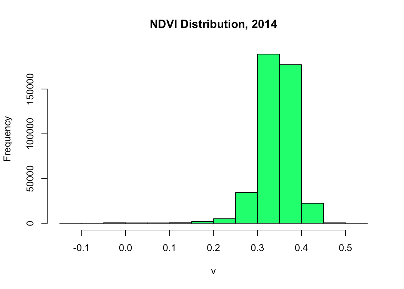

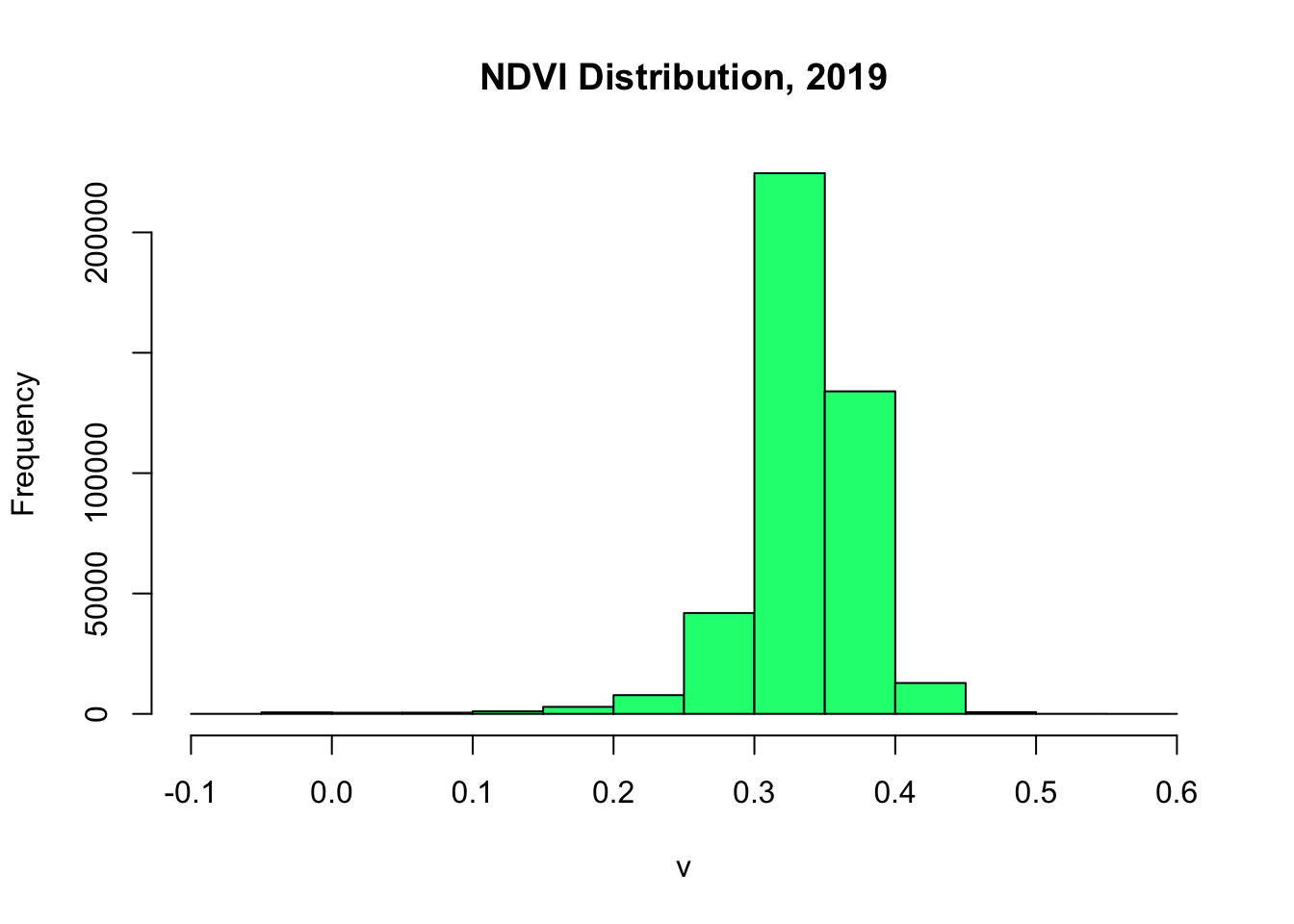
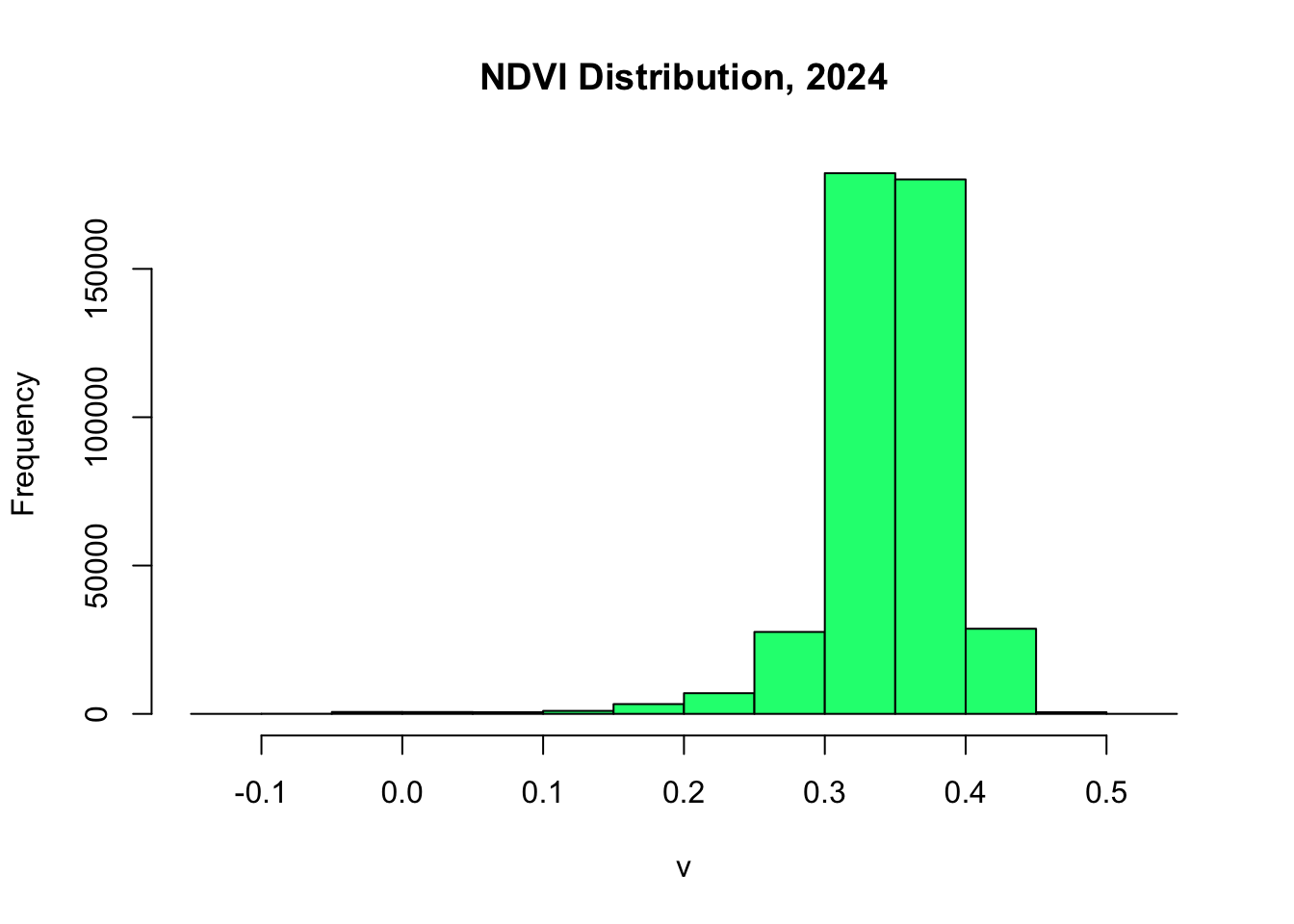
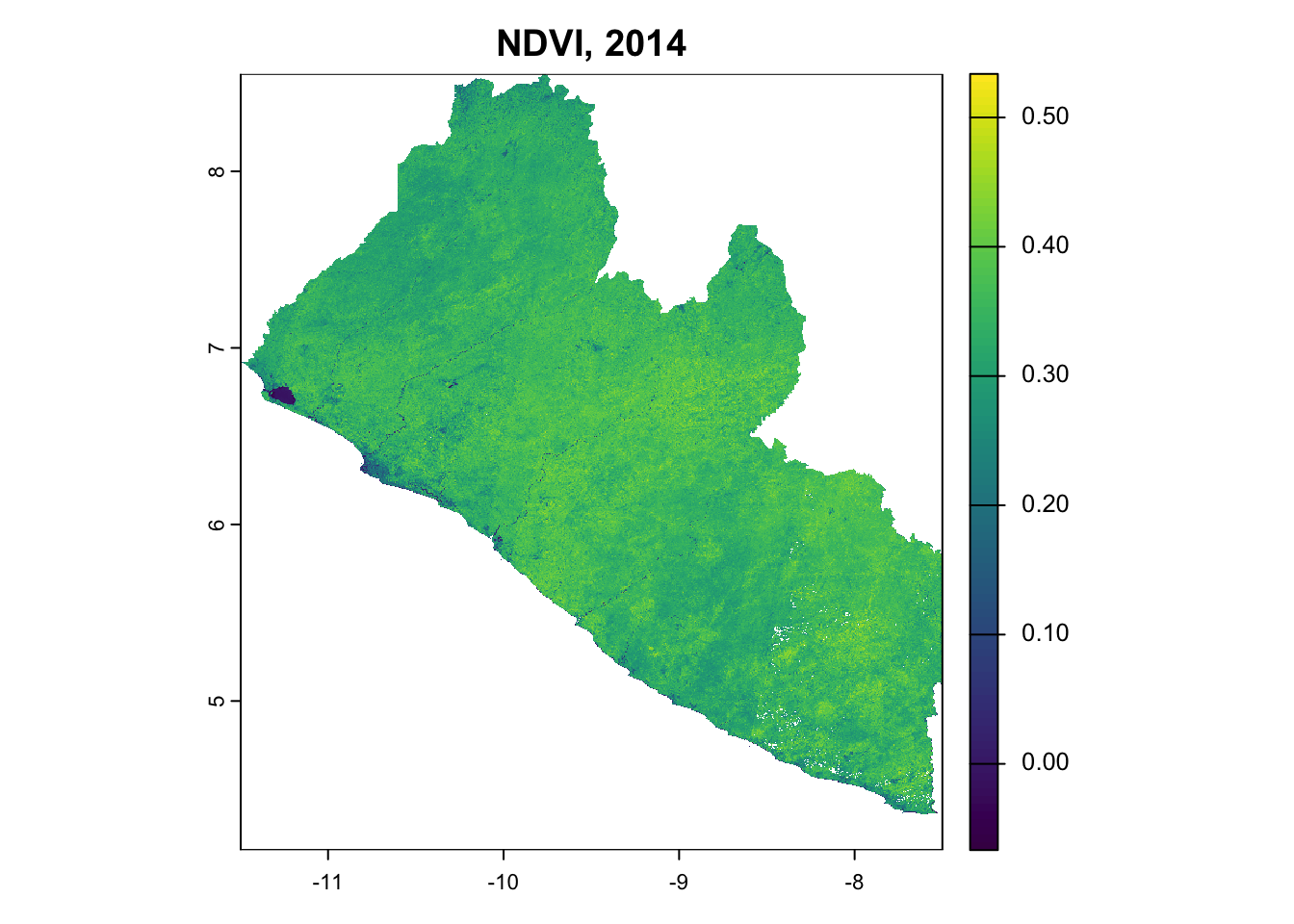
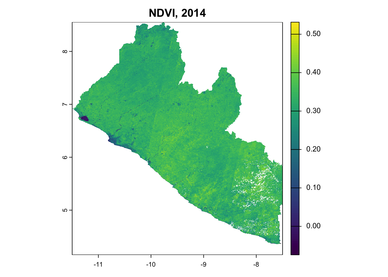
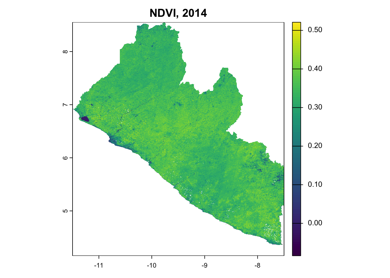
Figure 2: Multi-temporal satellite composites showing NDVI composites across the baseline period.

Metadata QA/QC

Metadata extraction ensures data provenance and enables quality control throughout the processing workflow. This steps comes in handy before exporting large collections from earth engine to personal drive, such as this one (>10GB).

# confirm dates, scene IDs, band names of images
firstImage_2014 = collection_2014.first()
sceneId_2014 = firstImage_2014.get('system:index').getInfo()
print(f"Scene ID for collection_2014: {sceneId_2014}")

firstImage_2019 = collection_2019.first()
sceneId_2019 = firstImage_2019.get('system:index').getInfo()
print(f"Scene ID for collection_2019: {sceneId_2019}")

firstImage_2024 = collection_2024.first()
sceneId_2024 = firstImage_2024.get('system:index').getInfo()
print(f"Scene ID for collection_2024: {sceneId_2024}")

bandNames_2014 = composite_2014.bandNames().getInfo()
print(f"Band names: {bandNames_2014}")

bandNames_2019 = composite_2019.bandNames().getInfo()
print(f"Band names: {bandNames_2019}")

bandNames_2024 = composite_2024.bandNames().getInfo()
print(f"Band names: {bandNames_2024}")

Scene ID for collection_2014: LC08_198055_20140104
Scene ID for collection_2019: LC08_198055_20190102
Scene ID for collection_2024: LC08_198055_20240116
Band names: ['BLUE', 'GREEN', 'RED', 'NIR08', 'SWIR16', 'SWIR22', 'NDVI']
Band names: ['BLUE', 'GREEN', 'RED', 'NIR08', 'SWIR16', 'SWIR22', 'NDVI']
Band names: ['BLUE', 'GREEN', 'RED', 'NIR08', 'SWIR16', 'SWIR22', 'NDVI']

Results confirm consistent band availability and standardized naming conventions across all periods.

Export Rasters

Cloud-optimized GeoTIFF format ensures efficient data access and interoperability with downstream analysis tools. The following export workflow also implements systematic file naming conventions suitable for metadata parsing required in remote sensing packages.

from datetime import datetime

# extract pathrow and date from scene ID
def get_pathrow_date(image_collection):
  first_image = image_collection.first()
  scene_id = first_image.get('system:index').getInfo()
  parts = scene_id.split('_')
  pathrow = parts[1]
  date_str = parts[2]
  date_obj = datetime.strptime(date_str, '%Y%m%d')
  date = date_obj.strftime('%Y-%m-%d')
  return pathrow, date

# define export parameters
def define_export_params(image, pathrow, date, band_name):
  description = f'composite_{date}_{band_name if isinstance(band_name, str) else "RGB"}_export'[:100]
  return {
    'image': image.select(band_name),
    'description': description,
    'folder': 'VT0007-deforestation-map',
    'fileNamePrefix': f'LANDSAT_TM-ETM-OLI_{pathrow}_{band_name if isinstance(band_name, str) else "RGB"}_{date}',
    'scale': 30,
    'region': country.geometry(),
    'maxPixels': 1e13,
    'fileFormat': 'GeoTIFF',
    'formatOptions': {'cloudOptimized': True}
  }

# get pathrow and date for each collection
pathrow_2014, date_2014 = get_pathrow_date(collection_2014)
pathrow_2019, date_2019 = get_pathrow_date(collection_2019)
pathrow_2024, date_2024 = get_pathrow_date(collection_2024)

# get band names
bandNames_2014 = composite_2014.bandNames().getInfo()
bandNames_2019 = composite_2019.bandNames().getInfo()
bandNames_2024 = composite_2024.bandNames().getInfo()

# export to cloud bucket
for band_name in bandNames_2014:
    export_params_2014 = define_export_params(composite_2014, pathrow_2014, date_2014, band_name)
    task_2014 = ee.batch.Export.image.toDrive(**export_params_2014)
    task_2014.start()
    print(f"Exporting 2014 image for band {band_name}. Task ID: {task_2014.id}")

for band_name in bandNames_2019:
    export_params_2019 = define_export_params(composite_2019, pathrow_2019, date_2019, band_name)
    task_2019 = ee.batch.Export.image.toDrive(**export_params_2019)
    task_2019.start()
    print(f"Exporting 2019 image for band {band_name}. Task ID: {task_2019.id}")

for band_name in bandNames_2024:
    export_params_2024 = define_export_params(composite_2024, pathrow_2024, date_2024, band_name)
    task_2024 = ee.batch.Export.image.toDrive(**export_params_2024)
    task_2024.start()
    print(f"Exporting 2024 image for band {band_name}. Task ID: {task_2024.id}")

export_params_2014_rgb = define_export_params(composite_2014, pathrow_2014, date_2014, ['RED', 'GREEN', 'BLUE'])
export_params_2014_rgb['image'] = composite_2014.visualize(**rgbVis)
task_2014_rgb = ee.batch.Export.image.toDrive(**export_params_2014_rgb)
task_2014_rgb.start()
print(f"Exporting 2014 RGB image. Task ID: {task_2014_rgb.id}")

export_params_2019_rgb = define_export_params(composite_2019, pathrow_2019, date_2019, ['RED', 'GREEN', 'BLUE'])
export_params_2019_rgb['image'] = composite_2019.visualize(**rgbVis)
task_2019_rgb = ee.batch.Export.image.toDrive(**export_params_2019_rgb)
task_2019_rgb.start()
print(f"Exporting 2019 RGB image. Task ID: {task_2019_rgb.id}")

export_params_2024_rgb = define_export_params(composite_2024, pathrow_2024, date_2024, ['RED', 'GREEN', 'BLUE'])
export_params_2024_rgb['image'] = composite_2024.visualize(**rgbVis)
task_2024_rgb = ee.batch.Export.image.toDrive(**export_params_2024_rgb)
task_2024_rgb.start()
print(f"Exporting 2024 RGB image. Task ID: {task_2024_rgb.id}")

Exporting 2014 image for band BLUE. Task ID: IRDIBYVEMKUAVGKZQ5HXKPBC
Exporting 2014 image for band GREEN. Task ID: EEWSBCRWWKUPRQWV4TQZ3B6C
Exporting 2014 image for band RED. Task ID: WXC6RRPJFOILRBYH5C3WOKTP
Exporting 2014 image for band NIR08. Task ID: 6PKRX3FP7ABDPURUHPZYDPWE
Exporting 2014 image for band SWIR16. Task ID: XK6EE5UFGWCCG7QSIDKKTJF5
Exporting 2014 image for band SWIR22. Task ID: W57UBUFB7HRB3EKMLJHNEW6H
Exporting 2014 image for band NDVI. Task ID: ZY7IGAO2K3CIVCUGRXKDNXVA
Exporting 2019 image for band BLUE. Task ID: E3J5YYQM2ZI2HSRDCBPRBWI4
Exporting 2019 image for band GREEN. Task ID: XVQICHKGYHHCLCFS2H4DEVUK
Exporting 2019 image for band RED. Task ID: 7ISMPTUBERKDVN2OZ2DR7U56
Exporting 2019 image for band NIR08. Task ID: 5QGL7XCZ6QPT2NKXEZFKXIPR
Exporting 2019 image for band SWIR16. Task ID: 4TDZ3QLG3JXJ5DXGZIIPPQAX
Exporting 2019 image for band SWIR22. Task ID: SK4Q6PS6IXIVWUICHTRX55UL
Exporting 2019 image for band NDVI. Task ID: 4XWVQ4UNRFEA4JV25IL22THI
Exporting 2024 image for band BLUE. Task ID: BITRT6BI7PKM6P6Z3FWPTEEL
Exporting 2024 image for band GREEN. Task ID: 2VUH34ENCZVIAYSRD3BJQG2G
Exporting 2024 image for band RED. Task ID: 2U5PRUP3VUAJIIC6WPR7L4IG
Exporting 2024 image for band NIR08. Task ID: Y2M2FPLUNIDRRKMEYTWWDBPD
Exporting 2024 image for band SWIR16. Task ID: WPGNYNGXEOCB67CX6VGCPOLG
Exporting 2024 image for band SWIR22. Task ID: L43YZOYPUYVWUMGJCCHS46UA
Exporting 2024 image for band NDVI. Task ID: 3LRYV6LDKHOGQ2TJ4Z3FV4QT
Exporting 2014 RGB image. Task ID: WWHVXMWV2RUT5IKPZNVCFQLA
Exporting 2024 RGB image. Task ID: DA6UDTKJM5NG4QQHHLQ7S2KZ

The export generates 18 individual band files plus 2 RGB and 3 NDVI composites, totaling 23 data products spanning the 10-year baseline period. Each file maintains consistent 30-meter spatial resolution and geographic projection for seamless integration with subsequent analysis workflows.

Stack Rasters

BLUE_2014=terra::rast("./data/cube_2014/LANDSAT_TM-ETM-OLI_198055_BLUE_2014-01-04.tif") 
BLUE_2019=terra::rast("./data/cube_2019/LANDSAT_TM-ETM-OLI_198055_BLUE_2019-01-02.tif")
BLUE_2024=terra::rast("./data/cube_2024/LANDSAT_TM-ETM-OLI_198055_BLUE_2024-01-16.tif")
GREEN_2014=terra::rast("./data/cube_2014/LANDSAT_TM-ETM-OLI_198055_GREEN_2014-01-04.tif")
GREEN_2019=terra::rast("./data/cube_2019/LANDSAT_TM-ETM-OLI_198055_GREEN_2019-01-02.tif")
GREEN_2024=terra::rast("./data/cube_2024/LANDSAT_TM-ETM-OLI_198055_GREEN_2024-01-16.tif")
NIR08_2014=terra::rast("./data/cube_2014/LANDSAT_TM-ETM-OLI_198055_NIR08_2014-01-04.tif")
NIR08_2019=terra::rast("./data/cube_2019/LANDSAT_TM-ETM-OLI_198055_NIR08_2019-01-02.tif")
NIR08_2024=terra::rast("./data/cube_2024/LANDSAT_TM-ETM-OLI_198055_NIR08_2024-01-16.tif")
RED_2014=terra::rast("./data/cube_2014/LANDSAT_TM-ETM-OLI_198055_RED_2014-01-04.tif")
RED_2019=terra::rast("./data/cube_2019/LANDSAT_TM-ETM-OLI_198055_RED_2019-01-02.tif")
RED_2024=terra::rast("./data/cube_2024/LANDSAT_TM-ETM-OLI_198055_RED_2024-01-16.tif")
SWIR16_2014=terra::rast("./data/cube_2014/LANDSAT_TM-ETM-OLI_198055_SWIR16_2014-01-04.tif")
SWIR16_2019=terra::rast("./data/cube_2019/LANDSAT_TM-ETM-OLI_198055_SWIR16_2019-01-02.tif")
SWIR16_2024=terra::rast("./data/cube_2024/LANDSAT_TM-ETM-OLI_198055_SWIR16_2024-01-16.tif")
SWIR22_2014=terra::rast("./data/cube_2014/LANDSAT_TM-ETM-OLI_198055_SWIR22_2014-01-04.tif")
SWIR22_2019=terra::rast("./data/cube_2019/LANDSAT_TM-ETM-OLI_198055_SWIR22_2019-01-02.tif")
SWIR22_2024=terra::rast("./data/cube_2024/LANDSAT_TM-ETM-OLI_198055_SWIR22_2024-01-16.tif")
NDVI_2014=terra::rast("./data/cube_2014/LANDSAT_TM-ETM-OLI_198055_NDVI_2014-01-04.tif")*0.0001 
NDVI_2019=terra::rast("./data/cube_2019/LANDSAT_TM-ETM-OLI_198055_NDVI_2019-01-02.tif")*0.0001 
NDVI_2024=terra::rast("./data/cube_2024/LANDSAT_TM-ETM-OLI_198055_NDVI_2024-01-16.tif")*0.0001 
DEM=terra::rast("./data/DEM/DEM_SRTMGL1_1ARCSEC_30M.tif")

NDVI_2014 = terra::project(NDVI_2014, "EPSG:4326")
NDVI_2019 = terra::project(NDVI_2019, "EPSG:4326")
NDVI_2024 = terra::project(NDVI_2024, "EPSG:4326")

BLUE_2014 = terra::resample(BLUE_2014, NDVI_2014) |> raster::raster() 
BLUE_2019 = terra::resample(BLUE_2019, NDVI_2014) |> raster::raster() 
BLUE_2024 = terra::resample(BLUE_2024, NDVI_2014) |> raster::raster() 
GREEN_2014 = terra::resample(GREEN_2014, NDVI_2014) |> raster::raster() 
GREEN_2019 = terra::resample(GREEN_2019, NDVI_2014) |> raster::raster() 
GREEN_2024 = terra::resample(GREEN_2024, NDVI_2014) |> raster::raster() 
NIR08_2014 = terra::resample(NIR08_2014, NDVI_2014) |> raster::raster() 
NIR08_2019 = terra::resample(NIR08_2019, NDVI_2014) |> raster::raster() 
NIR08_2024 = terra::resample(NIR08_2024, NDVI_2014) |> raster::raster() 
RED_2014 = terra::resample(RED_2014, NDVI_2014) |> raster::raster() 
RED_2019 = terra::resample(RED_2019, NDVI_2014) |> raster::raster() 
RED_2024 = terra::resample(RED_2024, NDVI_2014) |> raster::raster() 
SWIR16_2014 = terra::resample(SWIR16_2014, NDVI_2014) |> raster::raster() 
SWIR16_2019 = terra::resample(SWIR16_2019, NDVI_2014) |> raster::raster() 
SWIR16_2024 = terra::resample(SWIR16_2024, NDVI_2014) |> raster::raster() 
SWIR22_2014 = terra::resample(SWIR22_2014, NDVI_2014) |> raster::raster() 
SWIR22_2019 = terra::resample(SWIR22_2019, NDVI_2014) |> raster::raster() 
SWIR22_2024 = terra::resample(SWIR22_2024, NDVI_2014) |> raster::raster()
NDVI_2014 = raster::raster(NDVI_2014) 
NDVI_2019 = raster::raster(NDVI_2019) 
NDVI_2024 = raster::raster(NDVI_2024) 

raster::writeRaster(BLUE_2014, "./data/STACK/BLUE_2014.tif", format = "GTiff", overwrite = T)
raster::writeRaster(BLUE_2019, "./data/STACK/BLUE_2019.tif", format = "GTiff", overwrite = T)
raster::writeRaster(BLUE_2024, "./data/STACK/BLUE_2024.tif", format = "GTiff", overwrite = T)
raster::writeRaster(GREEN_2014, "./data/STACK/GREEN_2014.tif", format = "GTiff", overwrite = T)
raster::writeRaster(GREEN_2019, "./data/STACK/GREEN_2019.tif", format = "GTiff", overwrite = T)
raster::writeRaster(GREEN_2024, "./data/STACK/GREEN_2024.tif", format = "GTiff", overwrite = T)
raster::writeRaster(NIR08_2014, "./data/STACK/NIR08_2014.tif", format = "GTiff", overwrite = T)
raster::writeRaster(NIR08_2019, "./data/STACK/NIR08_2019.tif", format = "GTiff", overwrite = T)
raster::writeRaster(NIR08_2024, "./data/STACK/NIR08_2024.tif", format = "GTiff", overwrite = T)
raster::writeRaster(RED_2014, "./data/STACK/RED_2014.tif", format = "GTiff", overwrite = T)
raster::writeRaster(RED_2019, "./data/STACK/RED_2019.tif", format = "GTiff", overwrite = T)
raster::writeRaster(RED_2024, "./data/STACK/RED_2024.tif", format = "GTiff", overwrite = T)
raster::writeRaster(SWIR16_2014, "./data/STACK/SWIR16_2014.tif", format = "GTiff",overwrite=T)
raster::writeRaster(SWIR16_2019, "./data/STACK/SWIR16_2019.tif", format = "GTiff",overwrite=T)
raster::writeRaster(SWIR16_2024, "./data/STACK/SWIR16_2024.tif", format = "GTiff",overwrite=T)
raster::writeRaster(SWIR22_2014, "./data/STACK/SWIR22_2014.tif", format = "GTiff",overwrite=T)
raster::writeRaster(SWIR22_2019, "./data/STACK/SWIR22_2019.tif", format = "GTiff",overwrite=T)
raster::writeRaster(SWIR22_2024, "./data/STACK/SWIR22_2024.tif", format = "GTiff",overwrite=T)
raster::writeRaster(NDVI_2014, "./data/STACK/NDVI_2014.tif", format = "GTiff", overwrite = T)
raster::writeRaster(NDVI_2019, "./data/STACK/NDVI_2019.tif", format = "GTiff", overwrite = T)
raster::writeRaster(NDVI_2024, "./data/STACK/NDVI_2024.tif", format = "GTiff", overwrite = T)

# https://github.com/tilezen/joerd/blob/master/docs/data-sources.md#what-is-the-ground-resolution
DEM=elevatr::get_elev_raster(aoi_country, z = 12) 
DEM=terra::rast("./data/DEM/DEM_SRTMGL1_1ARCSEC_30M.tif") |> terra::project(crs(NDVI_2014))
DEM=terra::resample(DEM, NDVI_2014)
DEM=terra::crop(DEM, NDVI_2014)
DEM=terra::mask(DEM, NDVI_2014)
DEM_raster=raster::raster(DEM)
raster::writeRaster(DEM_raster, "./data/STACK/DEM.tif", format = "GTiff", overwrite = T)

BLUE_2014=raster::raster("./data/STACK/BLUE_2014.tif")
BLUE_2019=raster::raster("./data/STACK/BLUE_2019.tif")
BLUE_2024=raster::raster("./data/STACK/BLUE_2024.tif")
GREEN_2014=raster::raster("./data/STACK/GREEN_2014.tif")
GREEN_2019=raster::raster("./data/STACK/GREEN_2019.tif")
GREEN_2024=raster::raster("./data/STACK/GREEN_2024.tif")
NIR08_2014=raster::raster("./data/STACK/NIR08_2014.tif")
NIR08_2019=raster::raster("./data/STACK/NIR08_2019.tif")
NIR08_2024=raster::raster("./data/STACK/NIR08_2024.tif")
RED_2014=raster::raster("./data/STACK/RED_2014.tif")
RED_2019=raster::raster("./data/STACK/RED_2019.tif")
RED_2024=raster::raster("./data/STACK/RED_2024.tif")
SWIR16_2014=raster::raster("./data/STACK/SWIR16_2014.tif")
SWIR16_2019=raster::raster("./data/STACK/SWIR16_2019.tif")
SWIR16_2024=raster::raster("./data/STACK/SWIR16_2024.tif")
SWIR22_2014=raster::raster("./data/STACK/SWIR22_2014.tif")
SWIR22_2019=raster::raster("./data/STACK/SWIR22_2019.tif")
SWIR22_2024=raster::raster("./data/STACK/SWIR22_2024.tif")
NDVI_2014=raster::raster("./data/STACK/NDVI_2014.tif")
NDVI_2019=raster::raster("./data/STACK/NDVI_2019.tif")
NDVI_2024=raster::raster("./data/STACK/NDVI_2024.tif")
DEM=raster::raster("./data/STACK/DEM.tif")

STACK = brick(NDVI_2014, NDVI_2019, NDVI_2024,
          BLUE_2014, BLUE_2019, BLUE_2024, 
          GREEN_2014, GREEN_2019, GREEN_2024,
          NIR08_2014, NIR08_2019, NIR08_2024, 
          RED_2014, RED_2019, RED_2024, 
          SWIR16_2014, SWIR16_2019, SWIR16_2024, 
          SWIR22_2014, SWIR22_2019, SWIR22_2024,
          DEM)

raster::writeRaster(STACK,
  "./assets/LULC/inputs/STACK/LANDSAT_TM-ETM-OLI_198055_STACK-&-DEM_2014-01-04_2024-01-16.tif",
  format = "GTiff", 
  bandorder = "BIL", 
  overwrite = T)

Image Classification

We trained a Random Forest model fitted with 500 decision trees. The dataset was partitioned using a 70:30 ratio which was which was trained using Monte Carlo resampling regime (k=100). Accuracy assessments were reported using a confusion matrix. Uncertainty metrics were then used to explore best subset of variables according to magnitude and performances of recursive modeling, which informed final model selection.

STACK=raster::brick("./assets/LULC/inputs/LANDSAT_TM-ETM-OLI_198055_STACK-&-DEM_2014-01-04_2024-01-16.tif")
names(STACK[[1]]) = "NDVI_2014"
names(STACK[[2]]) = "NDVI_2019"
names(STACK[[3]]) = "NDVI_2024"
names(STACK[[4]]) = "BLUE_2014"
names(STACK[[5]]) = "BLUE_2019"
names(STACK[[6]]) = "BLUE_2024"
names(STACK[[7]]) = "GREEN_2014"
names(STACK[[8]]) = "GREEN_2019"
names(STACK[[9]]) = "GREEN_2024"
names(STACK[[10]]) = "NIR08_2014"
names(STACK[[11]]) = "NIR08_2019"
names(STACK[[12]]) = "NIR08_2024"
names(STACK[[13]]) = "RED_2014"
names(STACK[[14]]) = "RED_2019"
names(STACK[[15]]) = "RED_2024"
names(STACK[[16]]) = "SWIR16_2014"
names(STACK[[17]]) = "SWIR16_2019"
names(STACK[[18]]) = "SWIR16_2024"
names(STACK[[19]]) = "SWIR22_2014"
names(STACK[[20]]) = "SWIR22_2019"
names(STACK[[21]]) = "SWIR22_2024"
names(STACK[[22]]) = "DEM"

# extract yearly layers
STACK_2014=subset(STACK, c("NDVI_2014","BLUE_2014","GREEN_2014","NIR08_2014",
                           "RED_2014","SWIR16_2014","SWIR22_2014","DEM"))
# extract signatures
signatures_2014 = raster::extract(STACK_2014, samples ,df=T) # watch for data formats
samples_signatures_2014 <- dplyr::inner_join(signatures_2014, samples, by=c("ID"="id"))
samples_signatures_2014$geometry <- NULL # set geometry to NULL for model training

# training-test split, p=0.7 -> 70% split
trainIndex_2014 <- caret::createDataPartition(samples_signatures_2014$ID,list=F,p=0.7)
trainData_2014  <- samples_signatures_2014[trainIndex_2014,]  
testData_2014   <- samples_signatures_2014[-trainIndex_2014,] 

# interpolate NAs with class-median-normalization (NAs -> missing cloud pixels)
trainData_2014 <- trainData_2014 |> group_by(label) |> mutate(across(where(is.numeric),
    ~ ifelse(is.na(.), median(., na.rm = TRUE), .))) |> ungroup()
testData_2014 <- testData_2014 |> group_by(label) |> mutate(across(where(is.numeric),
    ~ ifelse(is.na(.), median(., na.rm = TRUE), .))) |> ungroup()

# assign model variables
response  <- c("label")
predictors_2014 <- c(
  "NDVI_2014", "BLUE_2014", "GREEN_2014", "RED_2014", 
  "NIR08_2014", "SWIR16_2014", "SWIR22_2014", "DEM"
  )
# set training parameters
cv_regime <- caret::trainControl(
  method          = 'cv',
  number          = 10,
  savePredictions = T,
  verboseIter     = F
  )

# train classifier
rf_model_2014 <- caret::train(
  label~.,
  data = trainData_2014[, c(predictors_2014, "label")], # drop ID var
  trControl = cv_regime,
  method    = "rf", 
  metric    = 'Kappa', 
  ntree     = 500,
  tuneLength= 6,
  importance= T
  )

Accuracy Assessment

Results suggested a moderate concordance between observed and predicted classes with optimal model performance during cross-validation at mtry of 3. Overall statistics reported Kappa Index of 71.04%, Accuracy of 88.61% (0.95CI 84.46%, 95.71%), and a smaller No Information Rate of 0.8158 (p<0.01). In addition, key classes of Forest were predicted with robust Sensitivity (98.92%) and Specificity (76.16%).

To address model weaknesses, the team recommends sourcing additional verified training samples, or alternatively applying a weighted Random Forest, Gradient Boosting or Support Vector Machines kernels (SVM) to improve performance of underrepresented classes. Note, these modeling updates will require substantial runtimes.

rf_test_2014 <- predict(rf_model_2014, testData_2014)
print(rf_model_2014) # cv results
caret::confusionMatrix(rf_test_2014,testData_2014$label) # blind test results

Random Forest 

1862 samples
   8 predictor
   7 classes: 'Bareground', 'Farmbush', 'Forest', 'Regrowth', 'Swamp', 'Urban', 'Water' 

No pre-processing
Resampling: Repeated Train/Test Splits Estimated (100 reps, 75%) 
Summary of sample sizes: 1399, 1399, 1399, 1399, 1399, 1399, ... 
Resampling results across tuning parameters:

  mtry  Accuracy   Kappa    
  2     0.9976674  0.9935532
  3     0.9976674  0.9935535
  4     0.9976674  0.9935553
  5     0.9976674  0.9935596
  6     0.9976674  0.9935626
  8     0.9976674  0.9935652

Kappa was used to select the optimal model using the largest value.
The final value used for the model was mtry = 8.
Confusion Matrix and Statistics

            Reference
Prediction   Bareground Farmbush Forest Regrowth Swamp Urban Water
  Bareground         28        8      0        0     0     3     0
  Farmbush            0       10      0        0     0     0     0
  Forest              4        0    696        8     0     0     0
  Regrowth            0        0      8       41     0     0     0
  Swamp               0        0      0        0    31     0     0
  Urban               0        4      0        0     0    80     0
  Water               0        0      0        0     0     0    10

Overall Statistics
                                          
               Accuracy : 0.9624          
                 95% CI : (0.9481, 0.9737)
    No Information Rate : 0.7562          
    P-Value [Acc > NIR] : < 2.2e-16       
                                          
                  Kappa : 0.9086        

 Mcnemar's Test P-Value : NA              

Statistics by Class:

                     Class: Bareground Class: Farmbush Class: Forest Class: Regrowth Class: Swamp Class: Urban
Sensitivity                    0.87500         0.45455        0.9886         0.83673       1.0000      0.96386
Specificity                    0.98776         1.00000        0.9471         0.99093       1.0000      0.99528
Pos Pred Value                 0.71795         1.00000        0.9831         0.83673       1.0000      0.95238
Neg Pred Value                 0.99552         0.98697        0.9641         0.99093       1.0000      0.99646
Prevalence                     0.03437         0.02363        0.7562         0.05263       0.0333      0.08915
Detection Rate                 0.03008         0.01074        0.7476         0.04404       0.0333      0.08593
Detection Prevalence           0.04189         0.01074        0.7605         0.05263       0.0333      0.09023
Balanced Accuracy              0.93138         0.72727        0.9679         0.91383       1.0000      0.97957
                     Class: Water
Sensitivity               1.00000
Specificity               1.00000
Pos Pred Value            1.00000
Neg Pred Value            1.00000
Prevalence                0.01074
Detection Rate            0.01074
Detection Prevalence      0.01074
Balanced Accuracy         1.00000

Model Calibration

We employed recursive predictor subsetting to identify predictors of greatest magnitude and non-informative features to enhance model performance and reduce model complexity, respectively. This aims to limit potential of multicollinearity, despite inherent robustness of randomForest algorithms against such violations. The subsetted model was evaluated on the test dataset. The confusion matrix and performance metrics are summarized below.

index_feature_2014 <- createMultiFolds(trainData_2014$label, times=5) 
predictor_seq_2014 <-seq(from=1, to=length(predictors_2014),by=2)
subset_regime_2014 <- rfeControl(
  method="LGOCV",
  number = 10,
  verbose=FALSE,
  functions=rfFuncs,
  index=index_feature_2014
  )

rf_model_subset_2014 <- caret::rfe(
  label~.,
  data = trainData_2014[, c(predictors_2014, "label")], 
  sizes = predictor_seq_2014,
  metric = "Kappa",
  ntree=500,
  method="rf",
  rfeControl = subset_regime_2014
  )

rf_subset_test_2014 <- predict(rf_model_subset_2014,testData_2014)
print(rf_model_subset_2014)

Recursive feature selection
Outer resampling method: Repeated Train/Test Splits Estimated (50 reps, 75%) 
Resampling performance over subset size:

 Variables Accuracy  Kappa AccuracySD  KappaSD Selected
         1   0.9974 0.9929  0.0038035 0.010585         
         3   0.9991 0.9976  0.0019897 0.005519         
         5   0.9995 0.9985  0.0016258 0.004489         
         7   0.9999 0.9997  0.0007603 0.002113        *
         8   0.9998 0.9994  0.0010642 0.002957         

The top 5 variables (out of 7):
   BLUE_2014, NDVI_2014, NIR08_2014, SWIR22_2014, SWIR16_2014
caret::confusionMatrix(rf_subset_test_2014$pred,testData_2014$label)
Confusion Matrix and Statistics

            Reference
Prediction   Bareground Farmbush Forest Regrowth Swamp Urban Water
  Bareground         21        0      0        0     0     0     0
  Farmbush            0        0      0        0     0     0     0
  Forest              0       14    709       17    31    16     0
  Regrowth            0        0      0       24     0     0     0
  Swamp               0        0      0        0     0     0     0
  Urban               0       10      0        0     0    68     0
  Water               0        0      7        0     0     0    14

Overall Statistics
                                          
               Accuracy : 0.898           
                 95% CI : (0.8767, 0.9167)
    No Information Rate : 0.7691          
    P-Value [Acc > NIR] : < 2.2e-16       
                                          
                  Kappa : 0.7002          
                                          
 Mcnemar's Test P-Value : NA              

Statistics by Class:

                     Class: Bareground Class: Farmbush Class: Forest
Sensitivity                    1.00000         0.00000        0.9902
Specificity                    1.00000         1.00000        0.6372
Pos Pred Value                 1.00000             NaN        0.9009
Neg Pred Value                 1.00000         0.97422        0.9514
Prevalence                     0.02256         0.02578        0.7691
Detection Rate                 0.02256         0.00000        0.7615
Detection Prevalence           0.02256         0.00000        0.8453
Balanced Accuracy              1.00000         0.50000        0.8137
                     Class: Regrowth Class: Swamp Class: Urban Class: Water
Sensitivity                  0.58537       0.0000      0.80952      1.00000
Specificity                  1.00000       1.0000      0.98819      0.99237
Pos Pred Value               1.00000          NaN      0.87179      0.66667
Neg Pred Value               0.98126       0.9667      0.98124      1.00000
Prevalence                   0.04404       0.0333      0.09023      0.01504
Detection Rate               0.02578       0.0000      0.07304      0.01504
Detection Prevalence         0.02578       0.0000      0.08378      0.02256
Balanced Accuracy            0.79268       0.5000      0.89886      0.99618

The subset model achieved an Accuracy of 89. 8%. These metrics closely align with the results of the original model, suggesting minimal or no loss in predictive power despite using fewer predictors. Given that the reduction in complexity offered by the subsetted model does not provide significant benefits in this context, we would recommend proceeding with the original model to make spatial predictions. Modelling operations were then repeated for 2019 and 2024, which were visualized as the classified time series below.

LULC_LIBERIA_2014=terra::rast("./assets/LULC/outputs/LULC_LIBERIA_2014-01-04.tif")
LULC_LIBERIA_2019=terra::rast("./assets/LULC/outputs/LULC_LIBERIA_2019-01-02.tif")
LULC_LIBERIA_2024=terra::rast("./assets/LULC/outputs/LULC_LIBERIA_2024-01-16.tif")
code_dict <- data.frame(id = c(1, 2, 3, 4, 5, 6, 7),
  label = c("Bareground", "Farmbush", "Forest", "Regrowth", "Swamp", "Urban", "Water"))
levels(LULC_LIBERIA_2014) <- code_dict
levels(LULC_LIBERIA_2019) <- code_dict
levels(LULC_LIBERIA_2024) <- code_dict
voi = terra::vect(aoi_states)
LULC_PROJECT_2014 = terra::crop(LULC_LIBERIA_2014, voi, mask=T)
LULC_PROJECT_2019 = terra::crop(LULC_LIBERIA_2019, voi, mask=T)
LULC_PROJECT_2024 = terra::crop(LULC_LIBERIA_2024, voi, mask=T)
terra::plot(LULC_LIBERIA_2014, main="Land Cover, 2014")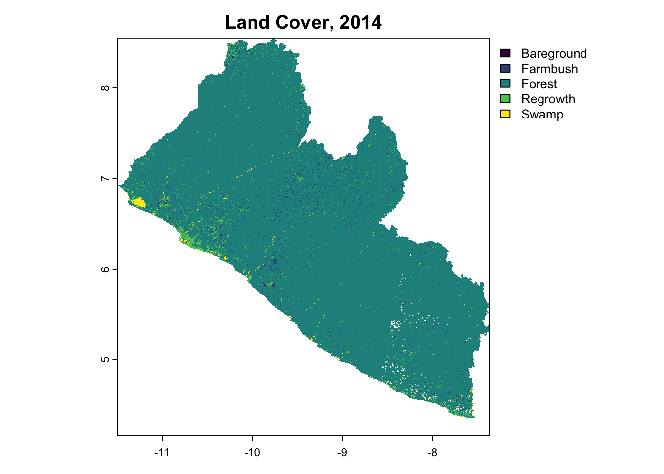

terra::plot(LULC_LIBERIA_2019, main="Land Cover, 2019")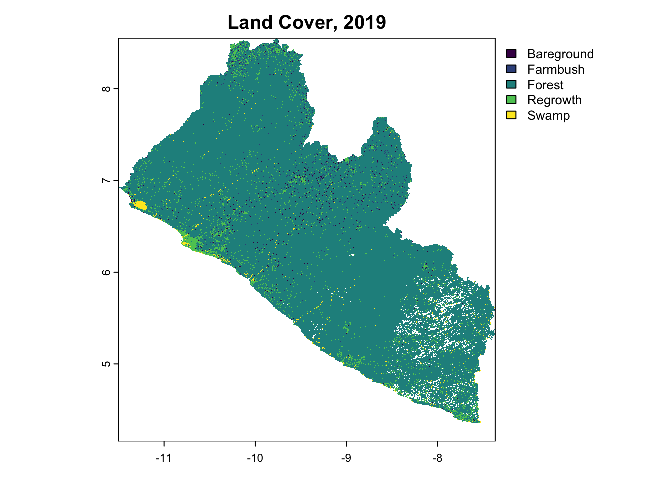

terra::plot(LULC_LIBERIA_2024, main="Land Cover, 2024")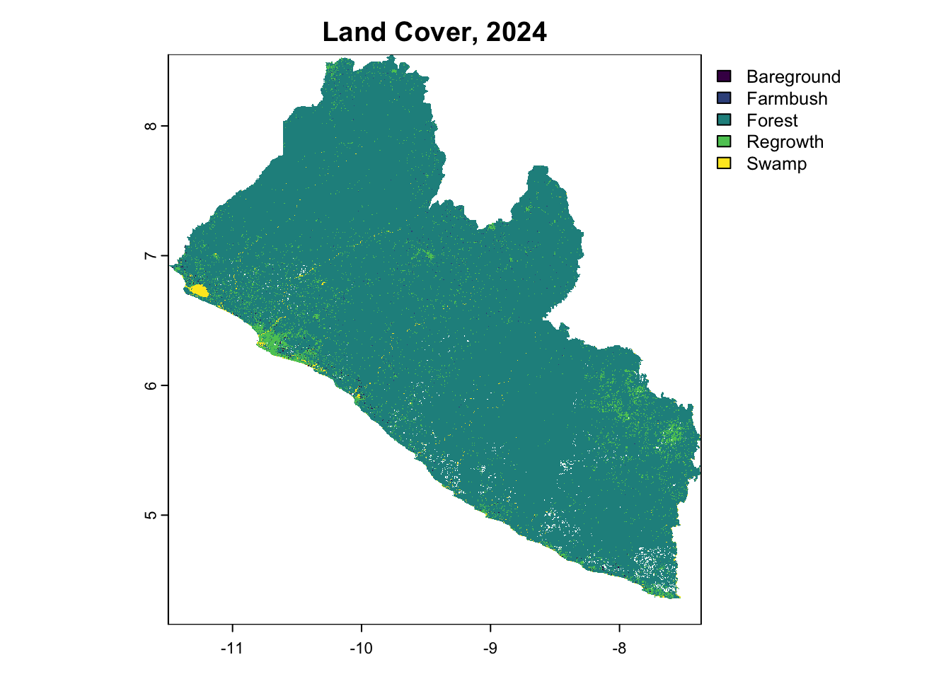

terra::plot(LULC_PROJECT_2014, main="Land Cover, 2014")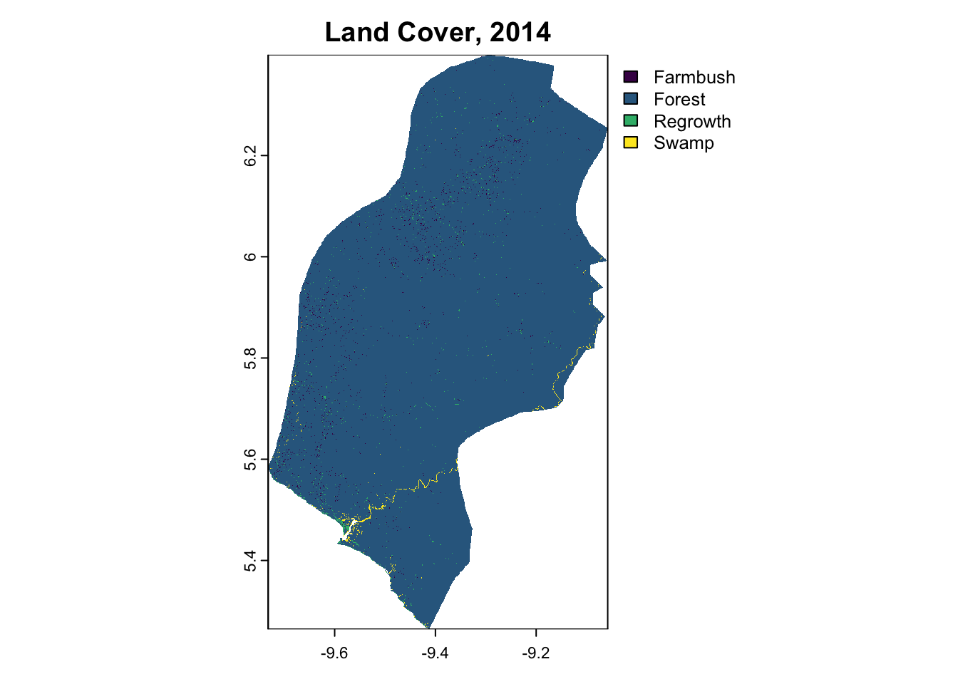

terra::plot(LULC_PROJECT_2019, main="Land Cover, 2019")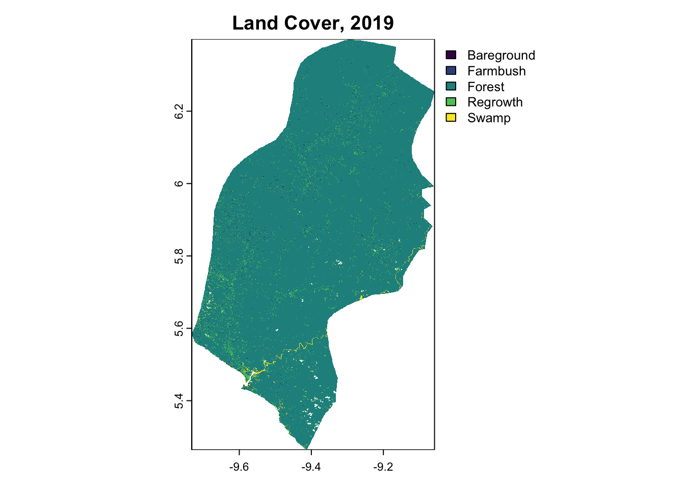

terra::plot(LULC_PROJECT_2024, main="Land Cover, 2024")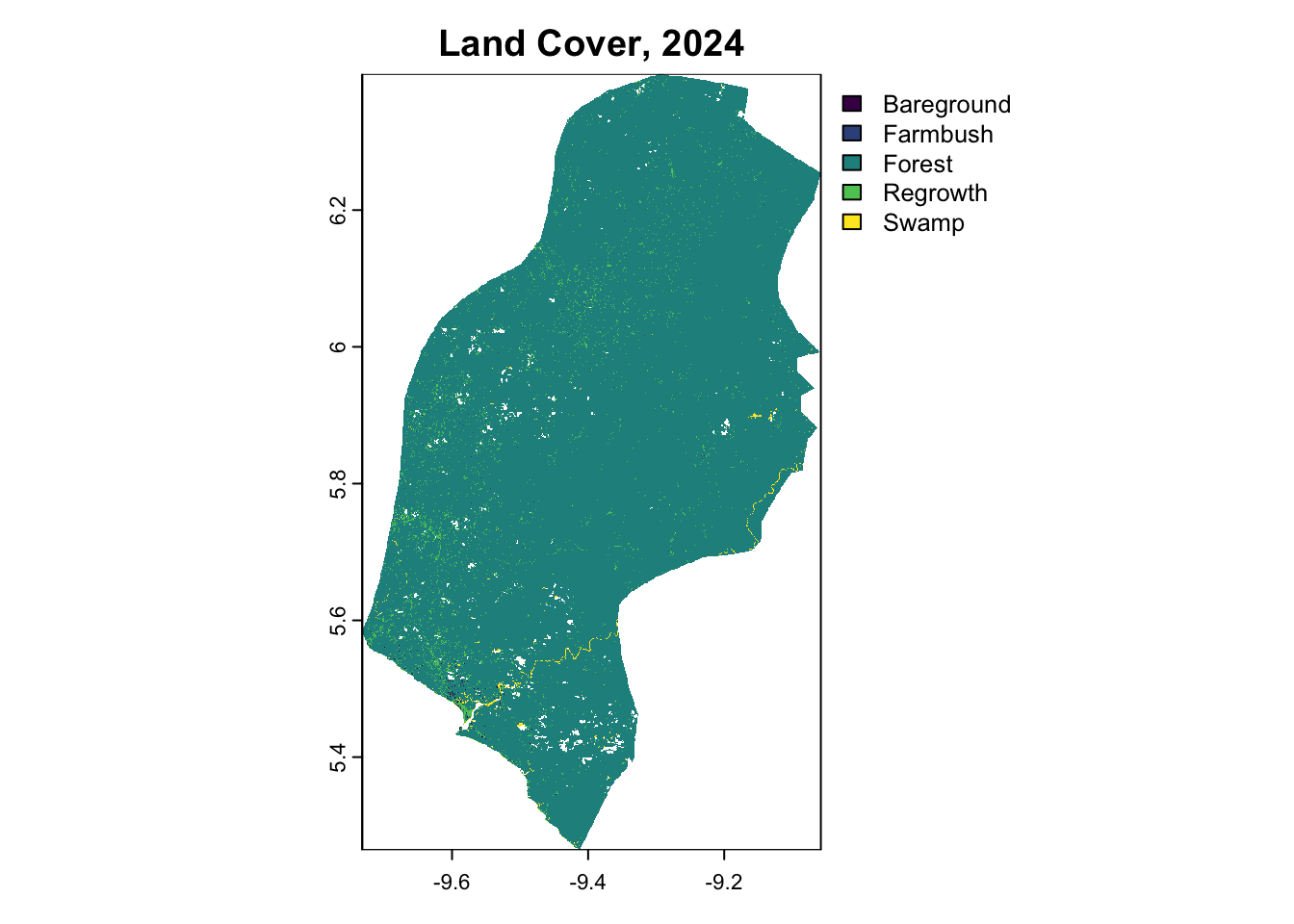

pixel_area_ha <- 0.088914  # 29.80124 x 29.80124 m² converted to hectares
compute_land_cover_summary <- function(aoi_states, rasters, pixel_area) {
  results = list()
  for (region in unique(aoi_states$NAME_1)) {
    for (year in names(rasters)) {
      cropped_raster = terra::crop(
        rasters[[year]], 
        aoi_states[aoi_states$NAME_1 == region, ], 
        mask = TRUE)
      freq = terra::freq(cropped_raster)
      freq$area_ha = freq$count * pixel_area
      freq$percentage = (freq$area_ha / sum(freq$area_ha)) * 100
      freq$region = region
      freq$year = year
      results[[paste(region, year, sep = "_")]] = freq
    }
  }
  do.call(rbind, results)
}

# Example call
rasters = list("2014" = LULC_PROJECT_2014, "2019" = LULC_PROJECT_2019, "2024" = LULC_PROJECT_2024)
land_cover_summary = compute_land_cover_summary(aoi_states, rasters, pixel_area_ha)
land_cover_summary

	layer	value	count	area_ha	percentage	region	year
Rivercess_2014.1	1	Bareground	2	1.778280e-01	0.0000336	Rivercess	2014
Rivercess_2014.2	1	Farmbush	45534	4.048610e+03	0.7657825	Rivercess	2014
Rivercess_2014.3	1	Forest	5847420	5.199175e+05	98.3408383	Rivercess	2014
Rivercess_2014.4	1	Regrowth	33254	2.956746e+03	0.5592597	Rivercess	2014
Rivercess_2014.5	1	Swamp	19865	1.766277e+03	0.3340859	Rivercess	2014
Rivercess_2019.1	1	Bareground	17152	1.525053e+03	0.2892307	Rivercess	2019
Rivercess_2019.2	1	Farmbush	3979	3.537888e+02	0.0670971	Rivercess	2019
Rivercess_2019.3	1	Forest	5717090	5.083293e+05	96.4061331	Rivercess	2019
Rivercess_2019.4	1	Regrowth	167842	1.492350e+04	2.8302857	Rivercess	2019
Rivercess_2019.5	1	Swamp	24151	2.147362e+03	0.4072534	Rivercess	2019
Rivercess_2024.1	1	Bareground	2841	2.526047e+02	0.0482377	Rivercess	2024
Rivercess_2024.2	1	Farmbush	3158	2.807904e+02	0.0536201	Rivercess	2024
Rivercess_2024.3	1	Forest	5736034	5.100137e+05	97.3928053	Rivercess	2024
Rivercess_2024.4	1	Regrowth	126894	1.128265e+04	2.1545484	Rivercess	2024
Rivercess_2024.5	1	Swamp	20660	1.836963e+03	0.3507886	Rivercess	2024

3. Results

Baseline Deforestation

# Reproject crs to enable metric area estimates
LULC_PROJECT_2014 = terra::project(LULC_PROJECT_2014, "EPSG:32629")
LULC_PROJECT_2019 = terra::project(LULC_PROJECT_2019, "EPSG:32629")
LULC_PROJECT_2024 = terra::project(LULC_PROJECT_2024, "EPSG:32629")

forest_class = 3
forest_2014 <- LULC_PROJECT_2014 == forest_class
forest_2019 <- LULC_PROJECT_2019 == forest_class
forest_2024 <- LULC_PROJECT_2024 == forest_class
forest_loss_2014_2019_gross <- forest_2014 & !forest_2019
forest_loss_2019_2024_gross <- forest_2019 & !forest_2024
forest_loss_2014_2024_gross <- forest_2014 & !forest_2024
forest_gain_2014_2019_gross <- !forest_2014 & forest_2019
forest_gain_2019_2024_gross <- !forest_2019 & forest_2024
forest_gain_2014_2024_gross <- !forest_2014 & forest_2024

# Forest net loss 
forest_loss_2014_2019 <- forest_loss_2014_2019_gross & !forest_gain_2014_2019_gross
forest_loss_2019_2024 <- forest_loss_2019_2024_gross & !forest_gain_2019_2024_gross
forest_loss_2014_2024 <- forest_loss_2014_2024_gross & !forest_gain_2014_2024_gross

# Save & visualize
raster::writeRaster(forest_2014, "./assets/LULC/outputs/forest_2014.tif",overwrite=T)
raster::writeRaster(forest_2019, "./assets/LULC/outputs/forest_2019.tif",overwrite=T)
raster::writeRaster(forest_2024, "./assets/LULC/outputs/forest_2024.tif",overwrite=T)
raster::writeRaster(forest_loss_2014_2019, "./assets/LULC/outputs//forest_loss_2014_2019.tif",overwrite=T)
raster::writeRaster(forest_loss_2019_2024, "./assets/LULC/outputs//forest_loss_2019_2024.tif",overwrite=T)
raster::writeRaster(forest_loss_2014_2024, "./assets/LULC/outputs//forest_loss_2014_2024.tif",overwrite=T)
resolution <- terra::res(forest_2014)[1]
forest_2014_estimate <- sum(forest_2014[], na.rm = TRUE) * resolution^2 / 10000
forest_2019_estimate <- sum(forest_2019[], na.rm = TRUE) * resolution^2 / 10000
forest_2024_estimate <- sum(forest_2024[], na.rm = TRUE) * resolution^2 / 10000
forest_loss_2014_2019_estimate <- sum(forest_loss_2014_2019[],na.rm=T)*resolution^2/10000
forest_loss_2019_2024_estimate <- sum(forest_loss_2019_2024[],na.rm=T)*resolution^2/10000
forest_loss_2014_2024_estimate <- sum(forest_loss_2014_2024[],na.rm=T)*resolution^2/10000

forest_summary <- data.frame(
  Year = c("2014", "2019", "2024", "Loss 2014-2024"),
  `Forest Area (hectares)` = c(
    format(forest_2014_estimate, big.mark = ",", digits = 1),
    format(forest_2019_estimate, big.mark = ",", digits = 1),
    format(forest_2024_estimate, big.mark = ",", digits = 1),
    format(forest_loss_2014_2024_estimate, big.mark = ",", digits = 1)
  )
)

options(scipen = 999)
knitr::kable(
  forest_summary, 
  caption = "Forest Cover Summary for Rivercress County",
  align = c("l", "r"))
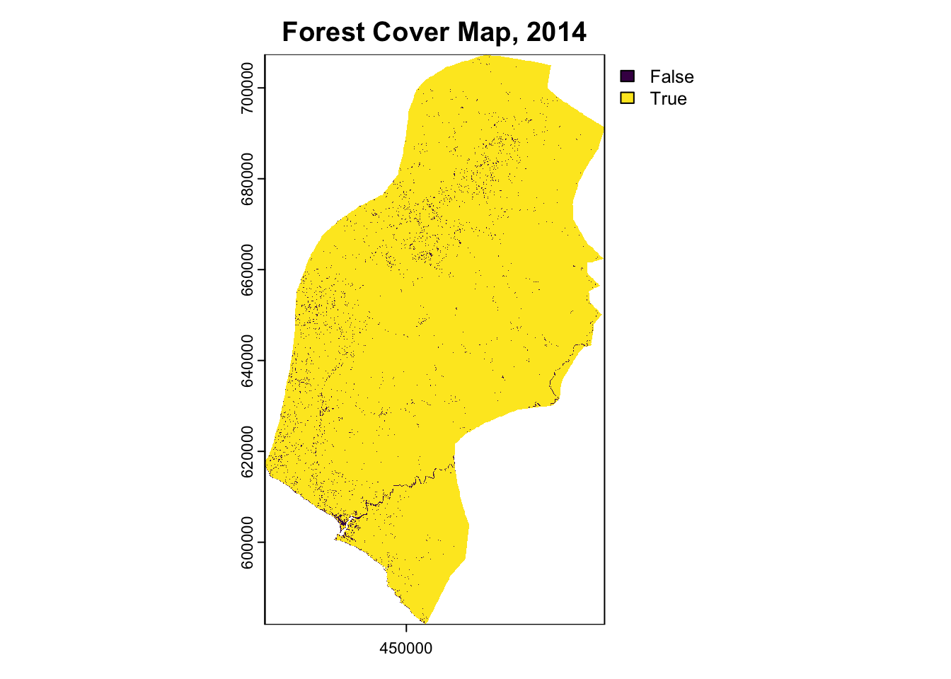
terra::plot(forest_2014, main="Forest Cover Map, 2014")
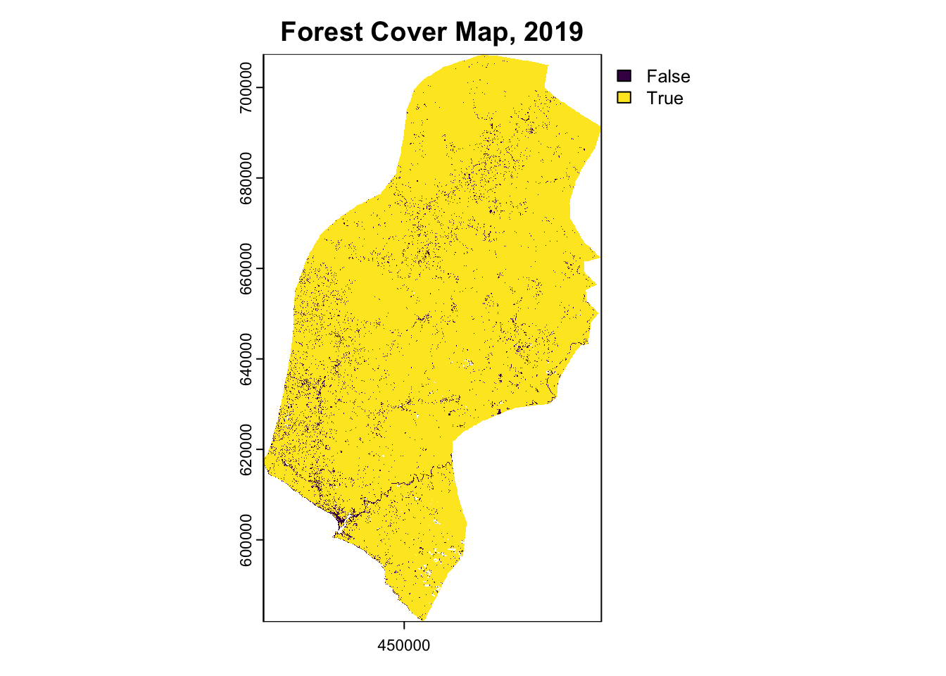
terra::plot(forest_2019, main="Forest Cover Map, 2019")
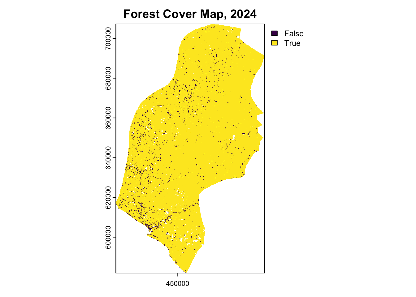
terra::plot(forest_2024, main="Forest Cover Map, 2024")
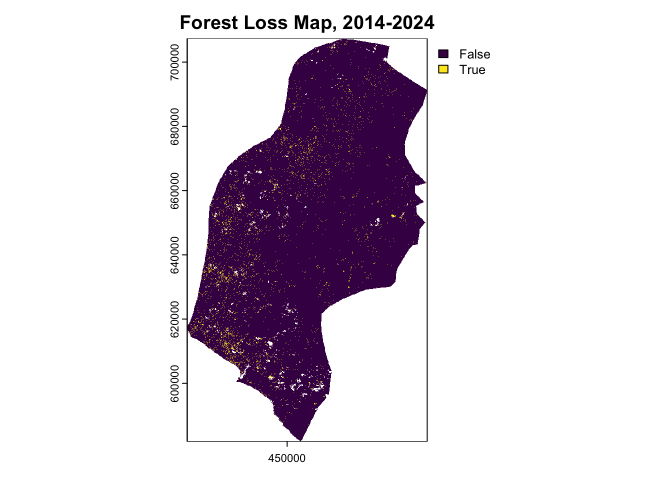
terra::plot(forest_loss_2014_2024, main="Forest Loss Map, 2014-2024")

Forest Cover Summary for Rivercress County
Year	Forest.Area..hectares.
2014	5e+05
2019	5e+05
2024	5e+05
Loss 2014-2024	10,883

Annualized Deforestation

# Assign zones
zones_sf = aoi_states |> sf::st_transform("EPSG:32629")
zones_sf$zone_id <- 1:nrow(zones_sf)
zones_sv <- terra::vect(zones_sf)

# Calculate zonal annualization by jurisdiction
forest_2024 = terra::rast("./assets/LULC/outputs/forest_2024.tif")
forest_loss_2014_2019 = terra::rast("./assets/LULC/outputs/forest_loss_2014_2019.tif")
forest_loss_2019_2024 = terra::rast("./assets/LULC/outputs/forest_loss_2019_2024.tif")
resolution <- terra::res(forest_loss_2014_2024) # 29.80244 * 29.80244
pixel_sqm <- (resolution[1] * resolution[2]) / 10000  # Convert m² to hectares

zonal_2014_2019 <- terra::extract(forest_loss_2014_2019,zones_sv,fun=sum,na.rm=T)
zonal_2019_2024 <- terra::extract(forest_loss_2019_2024,zones_sv,fun=sum,na.rm=T)
zonal_201_2024 <- terra::extract(forest_loss_2019_2024,zones_sv,fun=sum,na.rm=T)
names(zonal_2014_2019) <- c("zone_id", "loss_2014_2019")
names(zonal_2019_2024) <- c("zone_id", "loss_2019_2024")
zonal_2014_2019$loss_2014_2019 <- zonal_2014_2019$loss_2014_2019 * pixel_sqm
zonal_2019_2024$loss_2019_2024 <- zonal_2019_2024$loss_2019_2024 * pixel_sqm

# Merge baseline years
zonal_stats <- merge(
  zonal_2014_2019,
  zonal_2019_2024,
  by = "zone_id", 
  all = TRUE      
)

# Annualize 10-year total & rejoin to sf
zonal_stats$loss_10yr <- zonal_stats$loss_2014_2019 + zonal_stats$loss_2019_2024
zonal_stats$annual_loss_10yr <- zonal_stats$loss_10yr / 10
zones_sf <- merge(zones_sf, zonal_stats, by="zone_id", all.x=TRUE)
head(zones_sf[, c("zone_id", "loss_2014_2019", "loss_2019_2024", 
                  "loss_10yr", "annual_loss_10yr")])
zones_sv <- terra::vect(zones_sf)
annual_loss_10yr_raster <- rasterize(
  zones_sv,                  
  forest_loss_2014_2019,     
  field = "annual_loss_10yr")
names(annual_loss_10yr_raster) <- ("annual_loss_10yr")

raster::writeRaster(annual_loss_10yr_raster,
  "./assers/LULC/outputs/annual_loss_2014_2024_zonal.tif",overwrite=T)

tmap::tmap_mode("view")
tmap::tm_shape(deforestation_baseline) + 
  tmap::tm_raster("annual_loss_2014_2024_zonal.tif",title="Annual Deforestation (ha)") +
  tmap::tm_shape(aoi_states_all) + tmap::tm_borders(lwd = 1.2, col="black") +
  tmap::tm_text("NAME_1", just = "center", col="black", size=0.9) +
  tmap::tm_graticules(lines=T,labels.rot=c(0,90),lwd=0.2) +
  tmap::tm_scale_bar(position = c("RIGHT", "BOTTOM"), text.size = .5) + 
  tmap::tm_compass(color.dark = "gray60", text.color = "gray60", position = c("left", "top")) -> tm11

Baseline Emissions

The baseline emissions calculation for Rivercress County follows the Verra VM0048 methodology for REDD+ projects, utilizing carbon stock values derived from regional reference data. Carbon stock values were stratified according to forest management categories consistent with Community Forest designations.

Table 3: Carbon Stock Parameters for Rivercress County (tCO2 ha-1)

Carbon Pool	Community Forest	Post-Deforestation	∆ C Community Forest
Above-ground Biomass (CAB_Tree)	452.74	95.25	357.49
Below-ground Biomass (CBB_Tree)	108.64	25.73	82.91
Soil Organic Carbon (CSOC)	167.33	130.55	36.78
Total Carbon Stock Loss	728.71	251.53	477.18

Post-deforestation soil organic carbon stocks were calculated using IPCC 2006 Guidelines factors for land-use change from forest to agricultural systems:

Table 4: IPCC Soil Organic Carbon Factors

Parameter	Value	Definition	Source
F(Lu)	0.83	Stock change factor for land-use (forest to agriculture)	IPCC Chapter 5, Table 5.5
F(MG)	1.00	Management regime factor (full tillage)	IPCC Chapter 5, Table 5.5
F(I)	0.94	Input factor (low residue return)	IPCC Chapter 5, Table 5.5

Post-deforestation SOC = Pre-deforestation SOC × F(Lu) × F(MG) × F(I)
Post-deforestation SOC = 167.33 × 0.83 × 1.00 × 0.94 = 130.55 tCO2 ha-1

Baseline Emissions = Annual Deforestation Area × Carbon Stock Loss per Hectare**

Table 5: Baseline Emissions for Rivercress County

Component	Annual Area (ha)	Emission Factor (tCO2/ha)	Annual Emissions (tCO2)
Above-ground Biomass Loss	4,654	357.49	1,663,679
Below-ground Biomass Loss	4,654	82.91	385,874
Soil Organic Carbon Loss	4,654	36.78	171,210
Total Annual Baseline Emissions	4,654	477.18	2,220,763

Based on the land cover classification results from Section 2, the historical reference period (2014-2024) analysis for Rivercress County shows:

Table 6: Historical Forest Cover and Deforestation in Rivercress County

Metric	Value
Forest Area 2014	493,600 ha
Forest Area 2019	485,932 ha
Forest Area 2024	447,059 ha
Total Forest Loss (2014-2024)	46,541 ha
Average Annual Deforestation	4,654 ha/year
Annual Deforestation Rate	0.94%

Runtime Info

session_info.show()

-----
backports           NA
ee                  1.2.0
geemap              0.16.4
google              NA
ipyleaflet          0.19.2
numpy               1.26.4
session_info        1.0.0
-----
Click to view modules imported as dependencies
-----
IPython             7.34.0
jupyter_client      6.1.12
jupyter_core        5.7.2
jupyterlab          4.3.3
notebook            6.5.5
-----
Python 3.10.12 (main, Nov  6 2024, 20:22:13) [GCC 11.4.0]
Linux-6.1.85+-x86_64-with-glibc2.35
-----
Session information updated at 2024-12-15 22:22

devtools::session_info()

─ Session info ───────────────────────────────────────────────────────────────
 setting  value
 version  R version 4.3.0 (2023-04-21)
 os       macOS 15.6.1
 system   aarch64, darwin20
 ui       X11
 language (EN)
 collate  en_CA.UTF-8
 ctype    en_CA.UTF-8
 tz       America/Vancouver
 date     2025-08-27
 pandoc   3.7.0.2 @ /opt/local/bin/ (via rmarkdown)
 quarto   1.7.33 @ /usr/local/bin/quarto

─ Packages ───────────────────────────────────────────────────────────────────
 package           * version    date (UTC) lib source
 abind               1.4-8      2024-09-12 [1] CRAN (R 4.3.3)
 animation         * 2.7        2021-10-07 [1] CRAN (R 4.3.3)
 backports           1.5.0      2024-05-23 [1] CRAN (R 4.3.3)
 base64enc           0.1-3      2015-07-28 [1] CRAN (R 4.3.3)
 bibtex            * 0.5.1      2023-01-26 [1] CRAN (R 4.3.3)
 BIOMASS           * 2.2.4      2025-05-19 [1] CRAN (R 4.3.3)
 cachem              1.1.0      2024-05-16 [1] CRAN (R 4.3.3)
 cellranger          1.1.0      2016-07-27 [1] CRAN (R 4.3.0)
 chromote            0.5.1      2025-04-24 [1] CRAN (R 4.3.3)
 class               7.3-23     2025-01-01 [1] CRAN (R 4.3.3)
 classInt            0.4-11     2025-01-08 [1] CRAN (R 4.3.3)
 cli                 3.6.5      2025-04-23 [1] CRAN (R 4.3.3)
 codetools           0.2-20     2024-03-31 [1] CRAN (R 4.3.1)
 colorspace          2.1-1      2024-07-26 [1] CRAN (R 4.3.3)
 cols4all            0.8        2024-10-16 [1] CRAN (R 4.3.3)
 crosstalk           1.2.1      2023-11-23 [1] CRAN (R 4.3.3)
 data.table          1.17.8     2025-07-10 [1] CRAN (R 4.3.3)
 DBI                 1.2.3      2024-06-02 [1] CRAN (R 4.3.3)
 devtools            2.4.5      2022-10-11 [1] CRAN (R 4.3.0)
 dials               1.4.0      2025-02-13 [1] CRAN (R 4.3.3)
 DiceDesign          1.10       2023-12-07 [1] CRAN (R 4.3.3)
 dichromat           2.0-0.1    2022-05-02 [1] CRAN (R 4.3.3)
 digest              0.6.37     2024-08-19 [1] CRAN (R 4.3.3)
 dplyr             * 1.1.4      2023-11-17 [1] CRAN (R 4.3.1)
 e1071               1.7-16     2024-09-16 [1] CRAN (R 4.3.3)
 ellipsis            0.3.2      2021-04-29 [1] CRAN (R 4.3.3)
 evaluate            1.0.4      2025-06-18 [1] CRAN (R 4.3.3)
 extrafont         * 0.19       2023-01-18 [1] CRAN (R 4.3.3)
 extrafontdb         1.0        2012-06-11 [1] CRAN (R 4.3.3)
 farver              2.1.2      2024-05-13 [1] CRAN (R 4.3.3)
 fastmap             1.2.0      2024-05-15 [1] CRAN (R 4.3.3)
 forcats             1.0.0      2023-01-29 [1] CRAN (R 4.3.0)
 foreach             1.5.2      2022-02-02 [1] CRAN (R 4.3.3)
 fs                  1.6.6      2025-04-12 [1] CRAN (R 4.3.3)
 furrr               0.3.1      2022-08-15 [1] CRAN (R 4.3.0)
 future              1.40.0     2025-04-10 [1] CRAN (R 4.3.3)
 future.apply        1.11.3     2024-10-27 [1] CRAN (R 4.3.3)
 generics            0.1.4      2025-05-09 [1] CRAN (R 4.3.3)
 geodata           * 0.6-2      2024-06-10 [1] CRAN (R 4.3.3)
 ggplot2           * 3.5.2      2025-04-09 [1] CRAN (R 4.3.3)
 globals             0.17.0     2025-04-16 [1] CRAN (R 4.3.3)
 glue                1.8.0      2024-09-30 [1] CRAN (R 4.3.3)
 gower               1.0.2      2024-12-17 [1] CRAN (R 4.3.3)
 GPfit               1.0-9      2025-04-12 [1] CRAN (R 4.3.3)
 gridExtra           2.3        2017-09-09 [1] CRAN (R 4.3.3)
 gtable              0.3.6      2024-10-25 [1] CRAN (R 4.3.3)
 hardhat             1.4.1      2025-01-31 [1] CRAN (R 4.3.3)
 hms                 1.1.3      2023-03-21 [1] CRAN (R 4.3.0)
 htmltools         * 0.5.8.1    2024-04-04 [1] CRAN (R 4.3.3)
 htmlwidgets         1.6.4      2023-12-06 [1] CRAN (R 4.3.1)
 httpuv              1.6.16     2025-04-16 [1] CRAN (R 4.3.3)
 ipred               0.9-15     2024-07-18 [1] CRAN (R 4.3.3)
 iterators           1.0.14     2022-02-05 [1] CRAN (R 4.3.3)
 janitor           * 2.2.1      2024-12-22 [1] CRAN (R 4.3.3)
 jquerylib           0.1.4      2021-04-26 [1] CRAN (R 4.3.3)
 jsonlite            2.0.0      2025-03-27 [1] CRAN (R 4.3.3)
 kableExtra        * 1.4.0      2024-01-24 [1] CRAN (R 4.3.1)
 KernSmooth          2.23-26    2025-01-01 [1] CRAN (R 4.3.3)
 knitr             * 1.50       2025-03-16 [1] CRAN (R 4.3.3)
 later               1.4.2      2025-04-08 [1] CRAN (R 4.3.3)
 lattice             0.22-7     2025-04-02 [1] CRAN (R 4.3.3)
 lava                1.8.1      2025-01-12 [1] CRAN (R 4.3.3)
 leafem              0.2.4      2025-05-01 [1] CRAN (R 4.3.3)
 leaflegend          1.2.1      2024-05-09 [1] CRAN (R 4.3.3)
 leaflet             2.2.2      2024-03-26 [1] CRAN (R 4.3.1)
 leaflet.providers   2.0.0      2023-10-17 [1] CRAN (R 4.3.3)
 leafsync            0.1.0      2019-03-05 [1] CRAN (R 4.3.0)
 lhs                 1.2.0      2024-06-30 [1] CRAN (R 4.3.3)
 lifecycle           1.0.4      2023-11-07 [1] CRAN (R 4.3.3)
 listenv             0.9.1      2024-01-29 [1] CRAN (R 4.3.3)
 logger              0.4.0      2024-10-22 [1] CRAN (R 4.3.3)
 lubridate           1.9.4      2024-12-08 [1] CRAN (R 4.3.3)
 lwgeom              0.2-14     2024-02-21 [1] CRAN (R 4.3.1)
 magrittr            2.0.3      2022-03-30 [1] CRAN (R 4.3.3)
 maptiles            0.10.0     2025-05-07 [1] CRAN (R 4.3.3)
 MASS                7.3-60.0.1 2024-01-13 [1] CRAN (R 4.3.1)
 Matrix              1.6-5      2024-01-11 [1] CRAN (R 4.3.1)
 memoise             2.0.1      2021-11-26 [1] CRAN (R 4.3.3)
 microbenchmark      1.5.0      2024-09-04 [1] CRAN (R 4.3.3)
 mime                0.13       2025-03-17 [1] CRAN (R 4.3.3)
 miniUI              0.1.2      2025-04-17 [1] CRAN (R 4.3.3)
 minpack.lm          1.2-4      2023-09-11 [1] CRAN (R 4.3.3)
 nnet                7.3-20     2025-01-01 [1] CRAN (R 4.3.3)
 openxlsx          * 4.2.8      2025-01-25 [1] CRAN (R 4.3.3)
 pacman              0.5.1      2019-03-11 [1] CRAN (R 4.3.3)
 parallelly          1.45.0     2025-06-02 [1] CRAN (R 4.3.3)
 parsnip             1.3.2      2025-05-28 [1] CRAN (R 4.3.3)
 pillar              1.11.0     2025-07-04 [1] CRAN (R 4.3.3)
 pkgbuild            1.4.8      2025-05-26 [1] CRAN (R 4.3.3)
 pkgconfig           2.0.3      2019-09-22 [1] CRAN (R 4.3.3)
 pkgload             1.4.0      2024-06-28 [1] CRAN (R 4.3.3)
 plyr                1.8.9      2023-10-02 [1] CRAN (R 4.3.3)
 png                 0.1-8      2022-11-29 [1] CRAN (R 4.3.3)
 processx            3.8.6      2025-02-21 [1] CRAN (R 4.3.3)
 prodlim             2025.04.28 2025-04-28 [1] CRAN (R 4.3.3)
 profvis             0.4.0      2024-09-20 [1] CRAN (R 4.3.3)
 PROJ              * 0.6.0      2025-04-03 [1] CRAN (R 4.3.3)
 proj4               1.0-15     2025-03-21 [1] CRAN (R 4.3.3)
 promises            1.3.3      2025-05-29 [1] CRAN (R 4.3.3)
 proxy               0.4-27     2022-06-09 [1] CRAN (R 4.3.3)
 ps                  1.9.1      2025-04-12 [1] CRAN (R 4.3.3)
 purrr               1.1.0      2025-07-10 [1] CRAN (R 4.3.0)
 R6                  2.6.1      2025-02-15 [1] CRAN (R 4.3.3)
 rappdirs            0.3.3      2021-01-31 [1] CRAN (R 4.3.3)
 raster              3.6-32     2025-03-28 [1] CRAN (R 4.3.3)
 RColorBrewer        1.1-3      2022-04-03 [1] CRAN (R 4.3.3)
 Rcpp                1.1.0      2025-07-02 [1] CRAN (R 4.3.3)
 recipes             1.3.1      2025-05-21 [1] CRAN (R 4.3.3)
 remotes             2.5.0      2024-03-17 [1] CRAN (R 4.3.3)
 reproj            * 0.7.0      2024-06-11 [1] CRAN (R 4.3.3)
 reticulate          1.42.0     2025-03-25 [1] CRAN (R 4.3.3)
 rlang               1.1.6      2025-04-11 [1] CRAN (R 4.3.3)
 rmarkdown           2.29       2024-11-04 [1] CRAN (R 4.3.3)
 rpart               4.1.24     2025-01-07 [1] CRAN (R 4.3.3)
 rsample             1.3.0      2025-04-02 [1] CRAN (R 4.3.3)
 rstudioapi          0.17.1     2024-10-22 [1] CRAN (R 4.3.3)
 Rttf2pt1            1.3.12     2023-01-22 [1] CRAN (R 4.3.3)
 s2                  1.1.9      2025-05-23 [1] CRAN (R 4.3.3)
 scales              1.4.0      2025-04-24 [1] CRAN (R 4.3.3)
 sessioninfo         1.2.3      2025-02-05 [1] CRAN (R 4.3.3)
 sf                * 1.0-22     2025-08-25 [1] Github (r-spatial/sf@3660edf)
 shiny               1.11.1     2025-07-03 [1] CRAN (R 4.3.3)
 snakecase           0.11.1     2023-08-27 [1] CRAN (R 4.3.0)
 sp                  2.2-0      2025-02-01 [1] CRAN (R 4.3.3)
 spacesXYZ           1.6-0      2025-06-06 [1] CRAN (R 4.3.3)
 stars               0.6-8      2025-02-01 [1] CRAN (R 4.3.3)
 stringi             1.8.7      2025-03-27 [1] CRAN (R 4.3.3)
 stringr             1.5.1      2023-11-14 [1] CRAN (R 4.3.1)
 survival            3.8-3      2024-12-17 [1] CRAN (R 4.3.3)
 svglite             2.2.1      2025-05-12 [1] CRAN (R 4.3.3)
 systemfonts         1.2.3      2025-04-30 [1] CRAN (R 4.3.3)
 terra             * 1.8-60     2025-07-21 [1] CRAN (R 4.3.0)
 textshaping         1.0.1      2025-05-01 [1] CRAN (R 4.3.3)
 tibble              3.3.0      2025-06-08 [1] CRAN (R 4.3.3)
 tidyr               1.3.1      2024-01-24 [1] CRAN (R 4.3.1)
 tidyselect          1.2.1      2024-03-11 [1] CRAN (R 4.3.1)
 timechange          0.3.0      2024-01-18 [1] CRAN (R 4.3.3)
 timeDate            4041.110   2024-09-22 [1] CRAN (R 4.3.3)
 tinytex           * 0.57       2025-04-15 [1] CRAN (R 4.3.3)
 tmap              * 4.1        2025-05-12 [1] CRAN (R 4.3.3)
 tmaptools         * 3.2        2025-01-13 [1] CRAN (R 4.3.3)
 tune              * 1.3.0      2025-02-21 [1] CRAN (R 4.3.3)
 units               0.8-7      2025-03-11 [1] CRAN (R 4.3.3)
 urlchecker          1.0.1      2021-11-30 [1] CRAN (R 4.3.3)
 useful            * 1.2.6.1    2023-10-24 [1] CRAN (R 4.3.1)
 usethis             3.1.0      2024-11-26 [1] CRAN (R 4.3.3)
 vctrs               0.6.5      2023-12-01 [1] CRAN (R 4.3.3)
 viridisLite         0.4.2      2023-05-02 [1] CRAN (R 4.3.3)
 webshot           * 0.5.5      2023-06-26 [1] CRAN (R 4.3.0)
 webshot2          * 0.1.2      2025-04-23 [1] CRAN (R 4.3.3)
 websocket           1.4.4      2025-04-10 [1] CRAN (R 4.3.3)
 withr               3.0.2      2024-10-28 [1] CRAN (R 4.3.3)
 wk                  0.9.4      2024-10-11 [1] CRAN (R 4.3.3)
 workflows           1.2.0      2025-02-19 [1] CRAN (R 4.3.3)
 xfun                0.53       2025-08-19 [1] CRAN (R 4.3.0)
 XML                 3.99-0.18  2025-01-01 [1] CRAN (R 4.3.3)
 xml2                1.3.8      2025-03-14 [1] CRAN (R 4.3.3)
 xtable              1.8-4      2019-04-21 [1] CRAN (R 4.3.3)
 yaml                2.3.10     2024-07-26 [1] CRAN (R 4.3.3)
 yardstick           1.3.2      2025-01-22 [1] CRAN (R 4.3.3)
 zip                 2.3.3      2025-05-13 [1] CRAN (R 4.3.3)

 [1] /Library/Frameworks/R.framework/Versions/4.3-arm64/Resources/library
 * ── Packages attached to the search path.

──────────────────────────────────────────────────────────────────────────────

References

Government of Liberia. 2019. “Liberia’s Forest Reference Emission Level Submission to the UNFCCC.”

Stanimirova, Radost, Katelyn Tarrio, Konrad Turlej, Kristina McAvoy, Sophia Stonebrook, Kai-Ting Hu, Paulo Arévalo, et al. 2023. “A Global Land Cover Training Dataset from 1984 to 2020.” Scientific Data 10 (1): 879. https://doi.org/10.1038/s41597-023-02798-5.

Verra. 2021. “VT0007 Unplanned Deforestation Allocation Tool.”