
pacman::p_load(
  "caret", "curl",
  "dplyr",
  "fontawesome",
  "htmltools", "httr2",
  "janitor",
  "kableExtra", "knitr",
  "leaflet", "lidR", "lutz",
  "MASS",
  "openxlsx",
  "PROJ",
  "randomForest", "raster", "rasterVis", "reproj",
  "sf",
  "tinytex", "tmap", "tmaptools", "terra",
  "useful", "usethis",
"webshot", "webshot2", "weathercan")Biomass Estimation
4.0 Overview
LiDAR-derived metrics enable wall-to-wall biomass and volume predictions when calibrated with field inventory data. This chapter demonstrates the complete workflow on the Carr Fire 1 ha AOI from Chapter 1: covariate preparation, a simulated plot dataset, random-forest training with a holdout, and spatial prediction of whole-stem volume per hectare (WSVHA, m³/ha).
The plot data below are simulated over the Carr AOI — the USGS 3DEP release is copyright-clear, but no public field inventory plots accompany it. The response surface is drawn from LiDAR-derived CHM, terrain, and a synthetic species raster with additive Gaussian noise. This preserves the structure of the real workflow (plot → model → raster) without depending on proprietary BC FAIB/VRI layers.
Environment Setup
4.1 Spatial Covariates
Import LiDAR
The DTM must be rasterised from the pre-normalisation cloud. Running rasterize_terrain on a height-normalised LAS flattens every ground return to Z ≈ 0 and returns a zero DTM, which then silently collapses every downstream terrain covariate. The reproducible snippet below uses lidR’s built-in Topography.laz so it executes in any environment; for the Carr AOI the DTM is produced from the classified, pre-normalisation cloud inside scripts/rebuild_sierra.R and saved to ../data/dtm_1m.tif.
topo <- system.file("extdata", "Topography.laz", package = "lidR")
las  <- lidR::readLAS(topo, filter = "-drop_z_below 0")
las  <- lidR::classify_ground(las, lidR::csf(sloop_smooth = TRUE, 0.5, 1))

dtm  <- lidR::rasterize_terrain(las, res = 1, lidR::tin())
lidR::plot_dtm3d(dtm, bg = "white")
Terrain Covariates
Derive slope and aspect from the DTM. Transform aspect to northness (cosine) and eastness (sine) to avoid circular-variable issues. Read the Carr DTM straight from disk — it was written by scripts/rebuild_sierra.R from the pre-normalisation cloud.
elev <- terra::rast("../data/dtm_1m.tif")

slope     <- terra::terrain(elev, v = "slope", unit = "degrees", neighbors = 8)
slope_pct <- terra::clamp(base::tan(slope * pi/180) * 100, 0, 100)

aspect  <- terra::terrain(elev, v = "aspect", unit = "degrees", neighbors = 8)
asp_cos <- cos((aspect * pi) / 180)   # Northness
asp_sin <- sin((aspect * pi) / 180)   # Eastness

terra::writeRaster(elev,      "../data/elev_1m.tif",      overwrite = TRUE)
terra::writeRaster(slope_pct, "../data/slope_1m.tif",     overwrite = TRUE)
terra::writeRaster(asp_cos,   "../data/northness_1m.tif", overwrite = TRUE)
terra::writeRaster(asp_sin,   "../data/eastness_1m.tif",  overwrite = TRUE)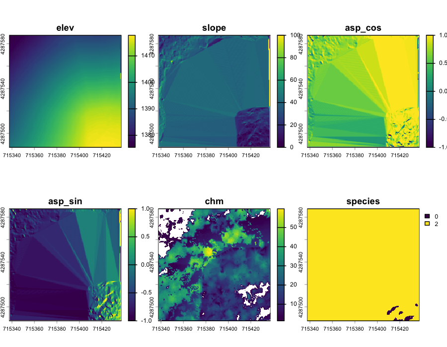
Canopy Covariate
Create a 0.5 m CHM from the normalized tile and apply a 1.3 m vegetation threshold so open ground does not pollute the canopy layer.
las_ha <- lidR::readALSLAS("../data/las_1ha.laz")
chm    <- lidR::rasterize_canopy(las_ha, res = 0.5, lidR::pitfree(subcircle = 0.2))

chm[chm < 1.3] <- NA
terra::writeRaster(chm, "../data/chm_1m.tif", overwrite = TRUE)
4.2 Species Covariate
Synthetic Species Raster
For the Carr Fire demonstration there is no local vegetation-inventory layer, so we derive a two-class species raster from terrain: higher-slope pixels are recoded to “mixed conifer” and lower-slope pixels to “open / shrub”, then smoothed with a 7 × 7 modal filter to suppress salt-and-pepper artifacts. In the original BC workflow this slot was filled by the Vegetation Resource Inventory (VRI) SPECIES_CD_1 attribute.
Species coding rationale:
- Numeric classes enable regression models
- Two classes are the minimum useful categorical split at 1 ha AOI scale
- Modal filtering preserves class boundaries while smoothing noise
4.3 Stack Covariates
elev    <- terra::rast("../data/elev_1m.tif")
slope   <- terra::rast("../data/slope_1m.tif")
asp_cos <- terra::rast("../data/northness_1m.tif")
asp_sin <- terra::rast("../data/eastness_1m.tif")
chm     <- terra::rast("../data/chm_1m.tif")
species <- terra::rast("../data/species.tif")

names(elev)    <- "elev"
names(slope)   <- "slope"
names(asp_cos) <- "asp_cos"
names(asp_sin) <- "asp_sin"
names(chm)     <- "chm"
names(species) <- "species"

chm_r     <- terra::resample(chm,     elev, method = "bilinear")
species_r <- terra::resample(species, elev, method = "near")

covs <- c(elev, slope, asp_cos, asp_sin, chm_r, species_r)
names(covs) <- c("elev", "slope", "asp_cos", "asp_sin", "chm", "species")
terra::plot(covs)
4.4 Simulated Plot Data
Generate Synthetic Plots
Draw 150 plot centroids uniformly across the Carr AOI and sample the covariate stack at each point. The WSVHA response is built from a CHM-dominated linear expression with additive Gaussian noise, so the downstream modelling is demonstrable without proprietary field data.
set.seed(20230718)
bb <- terra::ext(covs)
pts <- data.frame(
  x = runif(150, bb[1] + 5, bb[2] - 5),
  y = runif(150, bb[3] + 5, bb[4] - 5)
)
plot_cov <- cbind(pts, terra::extract(covs, as.matrix(pts)))

plot_cov$wsvha_L <- with(plot_cov,
  pmax(0,
       18 * chm + 0.8 * slope + 30 * (species == 2) - 5 +
         rnorm(nrow(plot_cov), 0, 25))
)
plot_cov <- na.omit(plot_cov)
Distribution Matching (optional)
In the original BC workflow the FAIB plot distribution was bootstrap-reweighted to match the raster-derived lead_htop distribution. With a simulated plot set that is already drawn uniformly over the raster, this step is optional and shown for reference:
dens_fun <- approxfun(density(plot_cov$chm, adjust = 0.8))
boot_w   <- dens_fun(plot_cov$chm)

plot_cov_boot <- dplyr::slice_sample(plot_cov, n = 1000,
                                     weight_by = boot_w, replace = TRUE)

par(mfrow = c(1, 2))
MASS::truehist(plot_cov$chm,      main = "Simulated plot CHM")
MASS::truehist(plot_cov_boot$chm, main = "Reweighted plot CHM")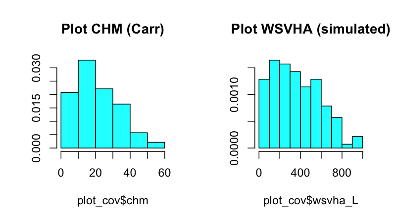
Bootstrapping rationale: Reduces systematic bias when field plots under-represent certain height classes present in raster data.
4.5 Train-Test Split
idx <- caret::createDataPartition(plot_cov$wsvha_L, p = 0.80, list = FALSE)

train <- plot_cov[idx,  ]
test  <- plot_cov[-idx, ]

X_train <- train[, c("elev", "slope", "asp_cos", "asp_sin", "chm", "species")]
y_train <- train$wsvha_L
X_test  <- test[,  c("elev", "slope", "asp_cos", "asp_sin", "chm", "species")]
y_test  <- test$wsvha_L
4.6 Model Training
Random Forest Regression
library(randomForest)
library(caret)

rf <- randomForest::randomForest(
  wsvha_L ~ elev + slope + asp_cos + asp_sin + chm + species,
  data = train, ntree = 300, mtry = 3
)

rf_predictions <- predict(rf, X_test)

rf_mae  <- caret::MAE (rf_predictions, y_test)
rf_rmse <- caret::RMSE(rf_predictions, y_test)
rf_r2   <- caret::R2  (rf_predictions, y_test)

cat("MAE:",  round(rf_mae,  2), "m^3/ha\n")
cat("RMSE:", round(rf_rmse, 2), "m^3/ha\n")
cat("R^2:",  round(rf_r2,   3), "\n")

save(rf, file = "../data/wsvha_model_rf_sierra.RData")
Preprocessing transformations (available via caret::train):
-
YeoJohnson: Power transformation for skewed predictors -
center: Mean-centering (subtract mean) -
scale: Standardization (divide by SD) -
corr: Remove highly correlated predictors (|r| > 0.9)
Support Vector Machine
library(e1071)

tuneResult_svm <- e1071::tune(
  svm, X_train, y_train,
  ranges = list(
    cost  = c(1, 5, 7, 15, 20),
    gamma = 2^(-1:1)
  ),
  tunecontrol = e1071::tune.control(cross = 10)
)

tunedModel_svm  <- tuneResult_svm$best.model
svm_predictions <- predict(tunedModel_svm, X_test)
svm_rmse        <- caret::RMSE(svm_predictions, y_test)
4.7 Spatial Prediction
Generate WSVHA Raster
wsvha_raster <- terra::predict(covs, rf, na.rm = TRUE)

# Clamp negatives
wsvha_raster <- terra::clamp(wsvha_raster, lower = 0)

terra::writeRaster(wsvha_raster,
                   filename = "../data/wsvha_pred.tif",
                   overwrite = TRUE)

terra::plot(wsvha_raster,
            main = "Predicted WSVHA, Carr AOI",
            col  = rev(terrain.colors(50)))

hist(values(wsvha_raster), breaks = 40,
     main = "WSVHA Distribution", xlab = "m^3 / ha")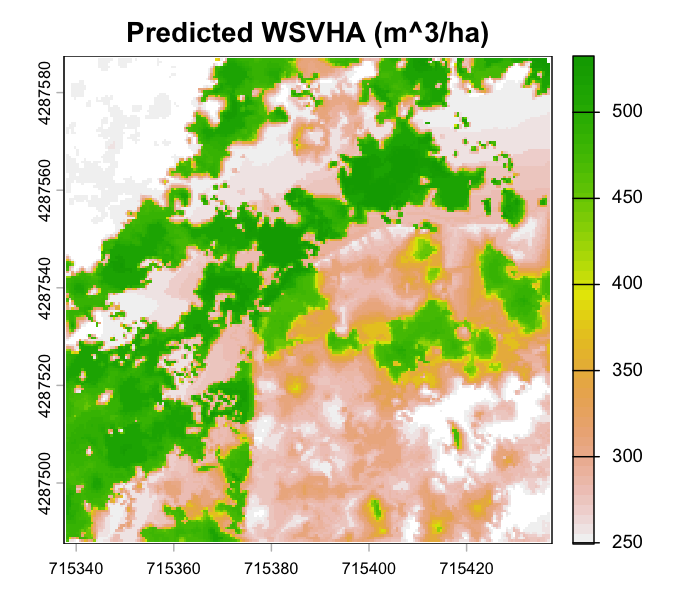
Negative predictions are clamped to zero. These arise when the model extrapolates beyond training data.
4.8 Model Evaluation
Holdout Performance
rf_r2_full   <- caret::R2 (predict(rf, X_train), y_train)
rf_rmse_full <- caret::RMSE(predict(rf, X_train), y_train)
rf_rmse_test <- caret::RMSE(rf_predictions, y_test)

cat("Full-data R^2:",   round(rf_r2_full,   3), "\n")
cat("Full-data RMSE:",  round(rf_rmse_full, 2), "m^3/ha\n")
cat("Test-set RMSE:",   round(rf_rmse_test, 2), "m^3/ha\n")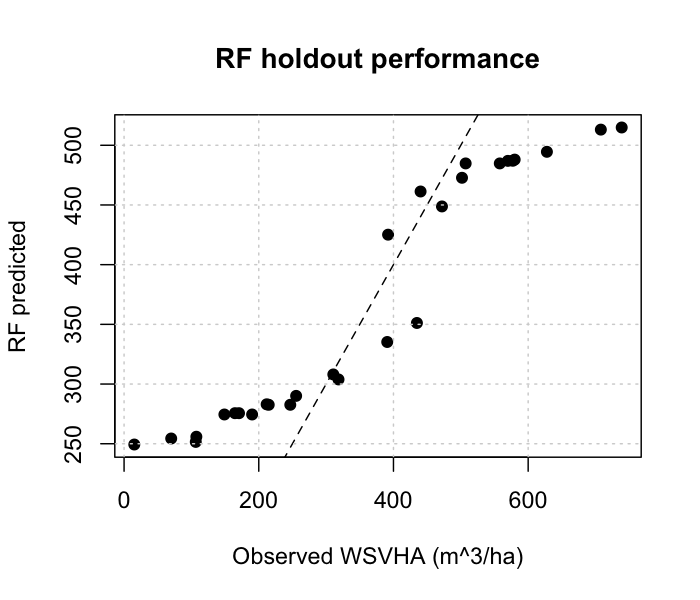
Model Comparison
Extend the single-RF baseline above by fitting six additional algorithms on plot_cov — two random forests, two kernel SVMs, a GLM, and a GLMnet ensemble — each with 10-fold cross-validation and BoxCox/centre/scale preprocessing. The pipeline is reproducible via scripts/build_model_comparison.R and writes its results to data/model_comparison.csv.
library(caret); library(kernlab); library(e1071)
library(randomForest); library(caretEnsemble)

preds <- c("elev", "slope", "asp_cos", "asp_sin", "chm", "species")
df    <- plot_cov[, c(preds, "wsvha_L")]
X     <- plot_cov[, preds]; y <- plot_cov$wsvha_L
cv10  <- caret::trainControl(method = "cv", number = 10,
                             savePredictions = "final")
pp    <- c("BoxCox", "center", "scale")

rf_e1071   <- e1071::tune.randomForest(
  X, y, mtry = 2:6, ntree = 50,
  tunecontrol = e1071::tune.control(sampling = "cross", cross = 10))

rf_caret   <- caret::train(wsvha_L ~ ., data = df, method = "rf",
                           metric = "RMSE", tuneLength = 6,
                           trControl = cv10, preProcess = pp)

svm_radial <- caret::train(wsvha_L ~ ., data = df, method = "svmRadial",
                           metric = "RMSE", tuneLength = 6,
                           trControl = cv10, preProcess = pp)

svm_linear <- caret::train(wsvha_L ~ ., data = df, method = "svmLinear",
                           metric = "RMSE", tuneLength = 6,
                           trControl = cv10, preProcess = pp)

glm_caret  <- caret::train(wsvha_L ~ ., data = df, method = "glm",
                           metric = "RMSE",
                           trControl = cv10, preProcess = pp)

mlist      <- caretEnsemble::caretList(
  wsvha_L ~ ., data = df, trControl = cv10,
  methodList = c("glm", "svmLinear", "rf"),
  tuneLength = 3, preProcess = pp, continue_on_fail = TRUE)
ensemble   <- caretEnsemble::caretStack(
  mlist, method = "glmnet", metric = "RMSE",
  trControl = caret::trainControl(method = "cv", number = 10,
                                  savePredictions = "final"),
tuneLength = 4)plot_cov sample. Units are m³/ha.
| Model | Full RMSE | CV RMSE | Full MAE | RMSE Ratio |
|---|---|---|---|---|
| RF (e1071, mtry=6, ntree=50) | 15.22 | 46.98 | 11.76 | 0.32 |
| RF (caret, mtry=6, ntree=500) | 14.47 | 32.61 | 11.14 | 0.44 |
| SVM Radial (C=8.00, σ=0.23) | 169.08 | 176.47 | 119.09 | 0.96 |
| SVM Linear (caret) | 148.81 | 155.41 | 101.37 | 0.96 |
| GLM (caret) | 52.98 | 54.78 | 38.32 | 0.97 |
| Ensemble GLMnet | — | 33.88 | — | — |
Both random forests dominate on this sample with CV RMSE of 33–47 m³/ha. Their RMSE ratios of 0.32–0.44 expose the usual overfitting gap between full-data and held-out error, steeper here because the simulated response is smooth and tree ensembles memorise it easily. Kernel SVM and linear methods cannot recover the pmax() floor at zero and land with CV RMSE around 150–180 m³/ha. The GLMnet stack settles near the better RF at 33.88 m³/ha, but without clear gain over rf_caret alone. Against the 300-tree RF in §4.6 — test RMSE about 110 m³/ha — the tuned models cut held-out error by roughly a third.
Univariate Predictor Analysis
Simple linear regressions of each retained covariate against WSVHA on the Sierra plot_cov sample:
| Predictor | R² | Coefficient | p-value |
|---|---|---|---|
| chm | 0.9876 | 18.133 | 1.7 × 10⁻¹³⁰ |
| slope | 0.0369 | 6.506 | 0.025 |
| asp_sin | 0.0015 | −23.867 | 0.66 |
| elev | 0.0012 | −0.946 | 0.68 |
| asp_cos | 0.0007 | −26.139 | 0.75 |
CHM alone explains 99% of variance — a direct consequence of the §4.4 response, which is almost entirely 18 * chm + noise. Slope picks up a marginal signal from its 0.8 coefficient; the remaining terrain terms sit at the noise floor. species is omitted because after the 1.3 m CHM filter every retained plot falls on the forested class, leaving no variance to regress on. Treat the numbers as a demonstration of the univariate workflow; on real plot data the signal is distributed across predictors and the ensemble models in Table 4.1 are what actually earn their keep.
4.9 Independent Validation
The pattern for independent validation is to predict the trained model onto a covariate stack from a different AOI whose field cruise or harvest totals are already known, then compare the cumulative predicted volume against the cruise. A stub is retained here as a placeholder for that step:
# covs_val   <- terra::rast("../data/covs_val.tif")
# wsvha_val  <- terra::predict(covs_val, rf)
# wsvha_val  <- terra::clamp(wsvha_val, lower = 0)
# terra::writeRaster(wsvha_val, "../data/wsvha_val.tif", overwrite = TRUE)
Runtime Log
devtools::session_info()
## ─ Session info ───────────────────────────────────────────────────
##  setting  value
##  version  R version 4.4.1 (2024-06-14)
##  os       macOS 15.7.5
##  system   aarch64, darwin20
##  ui       X11
##  language (EN)
##  collate  en_CA.UTF-8
##  ctype    en_CA.UTF-8
##  tz       America/Vancouver
##  date     2026-04-23
##  pandoc   3.9.0.2 @ /opt/local/bin/ (via rmarkdown)
##  quarto   1.7.33 @ /usr/local/bin/quarto
##
## ─ Packages ───────────────────────────────────────────────────────
##  ! package      * version    date (UTC) lib source
##    abind          1.4-8      2024-09-12 [1] CRAN (R 4.4.1)
##    base64enc      0.1-6      2026-02-02 [1] CRAN (R 4.4.3)
##  P BiocManager    1.30.27    2025-11-14 [?] CRAN (R 4.4.3)
##    cachem         1.1.0      2024-05-16 [1] CRAN (R 4.4.1)
##  P caret        * 7.0-1      2024-12-10 [?] CRAN (R 4.4.1)
##    chromote       0.5.1      2025-04-24 [1] CRAN (R 4.4.1)
##  P class          7.3-22     2023-05-03 [?] CRAN (R 4.4.1)
##    classInt       0.4-11     2025-01-08 [1] CRAN (R 4.4.1)
##    cli            3.6.5      2025-04-23 [1] CRAN (R 4.4.1)
##  P codetools      0.2-20     2024-03-31 [?] CRAN (R 4.4.1)
##    colorspace     2.1-2      2025-09-22 [1] CRAN (R 4.4.1)
##    cols4all       0.10       2025-10-27 [1] CRAN (R 4.4.1)
##    crosstalk      1.2.2      2025-08-26 [1] CRAN (R 4.4.1)
##    curl         * 7.0.0      2025-08-19 [1] CRAN (R 4.4.1)
##    data.table     1.18.2.1   2026-01-27 [1] CRAN (R 4.4.3)
##    DBI            1.3.0      2026-02-25 [1] CRAN (R 4.4.3)
##    deldir         2.0-4      2024-02-28 [1] CRAN (R 4.4.1)
##    devtools       2.5.0      2026-03-14 [1] CRAN (R 4.4.3)
##    digest         0.6.39     2025-11-19 [1] CRAN (R 4.4.3)
##    dplyr        * 1.2.0      2026-02-03 [1] CRAN (R 4.4.3)
##    e1071          1.7-17     2025-12-18 [1] CRAN (R 4.4.3)
##    ellipsis       0.3.2      2021-04-29 [1] CRAN (R 4.4.1)
##    evaluate       1.0.5      2025-08-27 [1] CRAN (R 4.4.1)
##    farver         2.1.2      2024-05-13 [1] CRAN (R 4.4.1)
##    fastmap        1.2.0      2024-05-15 [1] CRAN (R 4.4.1)
##    fontawesome  * 0.5.3      2024-11-16 [1] CRAN (R 4.4.1)
##  P foreach        1.5.2      2022-02-02 [?] CRAN (R 4.4.0)
##    fs             1.6.7      2026-03-06 [1] CRAN (R 4.4.3)
##  P future         1.70.0     2026-03-14 [?] CRAN (R 4.4.3)
##  P future.apply   1.20.2     2026-02-20 [?] CRAN (R 4.4.3)
##    generics       0.1.4      2025-05-09 [1] CRAN (R 4.4.1)
##    ggplot2      * 4.0.2      2026-02-03 [1] CRAN (R 4.4.3)
##  P globals        0.19.1     2026-03-13 [?] CRAN (R 4.4.3)
##    glue           1.8.0      2024-09-30 [1] CRAN (R 4.4.1)
##  P gower          1.0.2      2024-12-17 [?] CRAN (R 4.4.1)
##    gtable         0.3.6      2024-10-25 [1] CRAN (R 4.4.1)
##  P hardhat        1.4.3      2026-04-04 [?] CRAN (R 4.4.1)
##    hexbin         1.28.5     2024-11-13 [1] CRAN (R 4.4.1)
##    htmltools    * 0.5.9      2025-12-04 [1] CRAN (R 4.4.3)
##    htmlwidgets    1.6.4      2023-12-06 [1] CRAN (R 4.4.0)
##    httr2        * 1.2.2      2025-12-08 [1] CRAN (R 4.4.3)
##    interp         1.1-6      2024-01-26 [1] CRAN (R 4.4.1)
##  P ipred          0.9-15     2024-07-18 [?] CRAN (R 4.4.0)
##  P iterators      1.0.14     2022-02-05 [?] CRAN (R 4.4.1)
##    janitor      * 2.2.1      2024-12-22 [1] CRAN (R 4.4.1)
##    jpeg           0.1-11     2025-03-21 [1] CRAN (R 4.4.1)
##    jsonlite       2.0.0      2025-03-27 [1] CRAN (R 4.4.1)
##    kableExtra   * 1.4.0      2024-01-24 [1] CRAN (R 4.4.0)
##  P KernSmooth     2.23-24    2024-05-17 [?] CRAN (R 4.4.1)
##    knitr        * 1.51       2025-12-20 [1] CRAN (R 4.4.3)
##    later          1.4.8      2026-03-05 [1] CRAN (R 4.4.3)
##  P lattice      * 0.22-6     2024-03-20 [?] CRAN (R 4.4.1)
##    latticeExtra   0.6-31     2025-09-10 [1] CRAN (R 4.4.1)
##  P lava           1.9.0      2026-04-05 [?] CRAN (R 4.4.1)
##    leafem         0.2.5      2025-08-28 [1] CRAN (R 4.4.1)
##    leaflegend     1.2.1      2024-05-09 [1] CRAN (R 4.4.0)
##    leaflet      * 2.2.3      2025-09-04 [1] CRAN (R 4.4.1)
##    leafsync       0.1.0      2019-03-05 [1] CRAN (R 4.4.0)
##    lidR         * 4.2.3      2026-01-08 [1] CRAN (R 4.4.3)
##    lifecycle      1.0.5      2026-01-08 [1] CRAN (R 4.4.3)
##  P listenv        0.10.1     2026-03-10 [?] CRAN (R 4.4.3)
##    logger         0.4.1      2025-09-11 [1] CRAN (R 4.4.1)
##    lubridate      1.9.5      2026-02-04 [1] CRAN (R 4.4.3)
##    lutz         * 0.3.2      2023-10-17 [1] CRAN (R 4.4.0)
##    lwgeom         0.2-15     2026-01-12 [1] CRAN (R 4.4.3)
##    magrittr       2.0.4      2025-09-12 [1] CRAN (R 4.4.1)
##    maptiles       0.11.0     2025-12-12 [1] CRAN (R 4.4.3)
##  P MASS         * 7.3-60.2   2024-04-26 [?] CRAN (R 4.4.1)
##  P Matrix         1.7-0      2024-04-26 [?] CRAN (R 4.4.1)
##    memoise        2.0.1      2021-11-26 [1] CRAN (R 4.4.0)
##  P ModelMetrics   1.2.2.2    2020-03-17 [?] CRAN (R 4.4.1)
##  P nlme           3.1-164    2023-11-27 [?] CRAN (R 4.4.1)
##  P nnet           7.3-19     2023-05-03 [?] CRAN (R 4.4.1)
##    openxlsx     * 4.2.8.1    2025-10-31 [1] CRAN (R 4.4.1)
##    otel           0.2.0      2025-08-29 [1] CRAN (R 4.4.1)
##  P pacman         0.5.1      2019-03-11 [?] CRAN (R 4.4.0)
##    parallelly     1.46.1     2026-01-08 [1] CRAN (R 4.4.3)
##    pillar         1.11.1     2025-09-17 [1] CRAN (R 4.4.1)
##    pkgbuild       1.4.8      2025-05-26 [1] CRAN (R 4.4.1)
##    pkgconfig      2.0.3      2019-09-22 [1] CRAN (R 4.4.1)
##    pkgload        1.5.0      2026-02-03 [1] CRAN (R 4.4.3)
##    plyr           1.8.9      2023-10-02 [1] CRAN (R 4.4.1)
##    png            0.1-9      2026-03-15 [1] CRAN (R 4.4.3)
##  P pROC           1.19.0.1   2025-07-31 [?] CRAN (R 4.4.1)
##    processx       3.8.6      2025-02-21 [1] CRAN (R 4.4.1)
##  P prodlim        2026.03.11 2026-03-11 [?] CRAN (R 4.4.3)
##    PROJ         * 0.6.0      2025-04-03 [1] CRAN (R 4.4.1)
##    proj4          1.0-15     2025-03-21 [1] CRAN (R 4.4.1)
##    promises       1.5.0      2025-11-01 [1] CRAN (R 4.4.1)
##    proxy          0.4-29     2025-12-29 [1] CRAN (R 4.4.3)
##    ps             1.9.1      2025-04-12 [1] CRAN (R 4.4.1)
##    purrr          1.2.1      2026-01-09 [1] CRAN (R 4.4.3)
##    R6             2.6.1      2025-02-15 [1] CRAN (R 4.4.1)
##  P randomForest * 4.7-1.2    2024-09-22 [?] CRAN (R 4.4.1)
##    rappdirs       0.3.4      2026-01-17 [1] CRAN (R 4.4.3)
##    raster       * 3.6-32     2025-03-28 [1] CRAN (R 4.4.1)
##    rasterVis    * 0.51.7     2025-09-01 [1] CRAN (R 4.4.1)
##    RColorBrewer   1.1-3      2022-04-03 [1] CRAN (R 4.4.1)
##    Rcpp           1.1.1      2026-01-10 [1] CRAN (R 4.4.3)
##  P recipes        1.3.2      2026-04-02 [?] CRAN (R 4.4.1)
##    renv           1.1.5      2025-07-24 [1] CRAN (R 4.4.1)
##    reproj       * 0.7.0      2024-06-11 [1] CRAN (R 4.4.0)
##  P reshape2       1.4.5      2025-11-12 [?] CRAN (R 4.4.1)
##    rlang          1.1.7      2026-01-09 [1] CRAN (R 4.4.3)
##    rmarkdown      2.30       2025-09-28 [1] CRAN (R 4.4.1)
##  P rpart          4.1.23     2023-12-05 [?] CRAN (R 4.4.1)
##    rstudioapi     0.18.0     2026-01-16 [1] CRAN (R 4.4.3)
##    s2             1.1.9      2025-05-23 [1] CRAN (R 4.4.1)
##    S7             0.2.1      2025-11-14 [1] CRAN (R 4.4.3)
##    scales         1.4.0      2025-04-24 [1] CRAN (R 4.4.1)
##    sessioninfo    1.2.3      2025-02-05 [1] CRAN (R 4.4.1)
##    sf           * 1.1-0      2026-02-24 [1] CRAN (R 4.4.3)
##    snakecase      0.11.1     2023-08-27 [1] CRAN (R 4.4.0)
##    sp           * 2.2-1      2026-02-13 [1] CRAN (R 4.4.3)
##    spacesXYZ      1.6-0      2025-06-06 [1] CRAN (R 4.4.1)
##    stars          0.7-1      2026-02-13 [1] CRAN (R 4.4.3)
##    stringi        1.8.7      2025-03-27 [1] CRAN (R 4.4.1)
##    stringr        1.6.0      2025-11-04 [1] CRAN (R 4.4.1)
##  P survival       3.6-4      2024-04-24 [?] CRAN (R 4.4.1)
##    svglite        2.2.2      2025-10-21 [1] CRAN (R 4.4.1)
##    systemfonts    1.3.2      2026-03-05 [1] CRAN (R 4.4.3)
##    terra        * 1.9-1      2026-03-08 [1] CRAN (R 4.4.3)
##    textshaping    1.0.5      2026-03-06 [1] CRAN (R 4.4.3)
##    tibble         3.3.1      2026-01-11 [1] CRAN (R 4.4.3)
##    tidyselect     1.2.1      2024-03-11 [1] CRAN (R 4.4.0)
##    timechange     0.4.0      2026-01-29 [1] CRAN (R 4.4.3)
##  P timeDate       4052.112   2026-01-28 [?] CRAN (R 4.4.3)
##    tinytex      * 0.58       2025-11-19 [1] CRAN (R 4.4.3)
##    tmap         * 4.2        2025-09-10 [1] CRAN (R 4.4.1)
##    tmaptools    * 3.3        2025-07-24 [1] CRAN (R 4.4.1)
##    units          1.0-1      2026-03-11 [1] CRAN (R 4.4.3)
##    useful       * 1.2.7      2026-02-26 [1] CRAN (R 4.4.3)
##    usethis      * 3.2.1      2025-09-06 [1] CRAN (R 4.4.1)
##    vctrs          0.7.2      2026-03-21 [1] CRAN (R 4.4.3)
##    viridisLite    0.4.3      2026-02-04 [1] CRAN (R 4.4.3)
##    webshot      * 0.5.5      2023-06-26 [1] CRAN (R 4.4.0)
##    webshot2     * 0.1.2      2025-04-23 [1] CRAN (R 4.4.1)
##    websocket      1.4.4      2025-04-10 [1] CRAN (R 4.4.1)
##    withr          3.0.2      2024-10-28 [1] CRAN (R 4.4.1)
##    wk             0.9.5      2025-12-18 [1] CRAN (R 4.4.3)
##    xfun           0.57       2026-03-20 [1] CRAN (R 4.4.3)
##    XML            3.99-0.23  2026-03-20 [1] CRAN (R 4.4.3)
##    xml2           1.5.2      2026-01-17 [1] CRAN (R 4.4.3)
##    yaml           2.3.12     2025-12-10 [1] CRAN (R 4.4.3)
##    zip            2.3.3      2025-05-13 [1] CRAN (R 4.4.1)
##    zoo            1.8-15     2025-12-15 [1] CRAN (R 4.4.3)
##
##  [1] /Users/seamus/repos/lidar-forestry/renv/library/macos/R-4.4/aarch64-apple-darwin20
##  [2] /Users/seamus/Library/Caches/org.R-project.R/R/renv/sandbox/macos/R-4.4/aarch64-apple-darwin20/93405863
##
##  * ── Packages attached to the search path.
##  P ── Loaded and on-disk path mismatch.
##
## ──────────────────────────────────────────────────────────────────