Wildfire Emissions

Preface

---

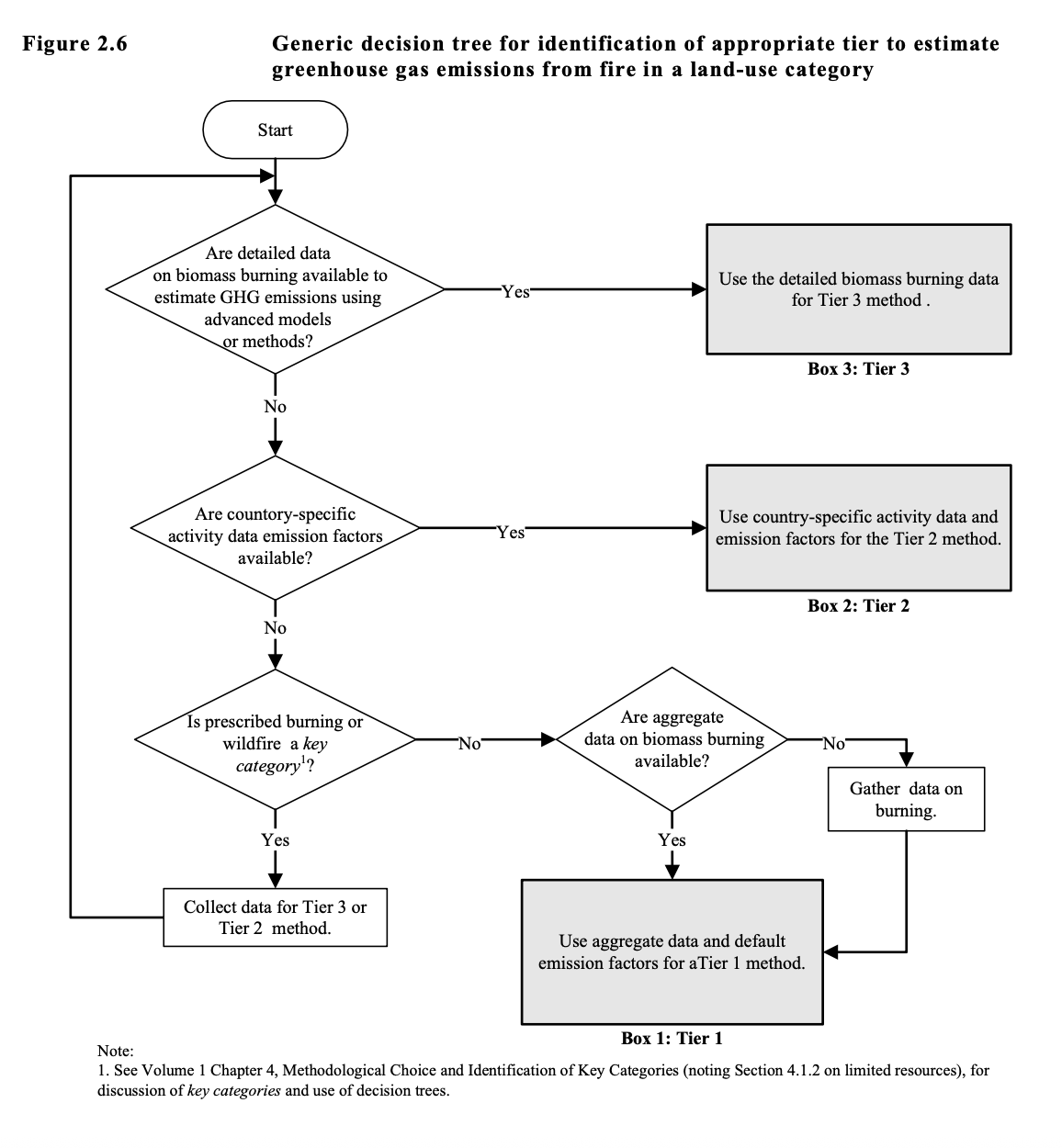
This eBook demonstrates the IPCC Tier 1 method for estimating greenhouse gas emissions from biomass burning, implementing Equation 2.27 from the 2019 IPCC Refinement (IPCC, 2019) end-to-end: satellite-based burned area detection, land cover stratification into fire categories, assignment of default fuel consumption values, and application of emission factors to derive CH₄, N₂O, and CO₂ estimates formatted for UNFCCC reporting. All workflows use Honduras as the example AOI. Paged links to source materials are provided in footnotes throughout.

Under the Managed Land Proxy (MLP), all fires on managed land — including natural wildfires — count toward a country’s reported LULUCF balance. The 2019 Refinement (Section 2.6) provides optional guidance for disaggregating natural disturbance spikes from background anthropogenic fire activity. This eBook implements both the standard Tier 1 calculation and the disaggregation framework, structured in four chapters:

1. Burned Area: Extract and validate burned area from MODIS MCD64A1, apply uncertainty filters, aggregate temporally, and compare against alternative fire products.
2. Fuel Stratification: Classify burned pixels into fire categories using land cover, climate zones, and soil classification.
3. Fuel Consumption: Assign IPCC default fuel consumption factors (M_B × C_f) by vegetation type and climate zone.
4. Emission Factors: Apply emission factors (G_ef) via Equation 2.27, compute CH₄ and N₂O emissions, and format for UNFCCC CRF reporting.

---

Tier 1 Stratification Datasets¹

• MODIS MCD64A1 C6.1: Monthly burned area (500 m, 2000–present). GEE: MODIS/061/MCD64A1. Bands: BurnDate, Uncertainty, QA.
• MODIS MCD12Q1 C6.1: IGBP annual land cover (500 m). GEE: MODIS/061/MCD12Q1. Band: LC_Type1.
• MODIS MOD14A1 C6.1: Daily thermal anomalies / active fires (1 km). GEE: MODIS/061/MOD14A1. Band: FireMask.
• IPCC Global Climate Regions: 12-zone classification derived per IPCC 2006 & 2019 guidelines, maintained by ESDAC and individual contributors.
• IPCC Global Soil Zones: 13-class soil classification from HWSD v2.0 via WRB-to-IPCC taxotransfer (Batjes, 2009; batjes2010ipcc?) (GEE Asset).
• FAO Agro-Ecological Zones: Climate-vegetation framework for fuel consumption stratification (V4, V5).
• FAO GAUL 2015: Administrative boundaries. GEE: FAO/GAUL/2015/level0, FAO/GAUL/2015/level1.

Validation Datasets

• Landsat 8 C2 T1 L2: Surface reflectance (30 m). Used for dNBR validation.
• Hansen Global Forest Change v1.12: Tree canopy cover 2000 (30 m).
• ESA WorldCover 2020 v100: Global land cover (10 m).
• WorldClim V1 Bioclimatic Variables: 1 km climatologies (bio01, bio12) for climate zone delineation.
• USGS SRTM DEM: 30 m elevation for lowland organic soil proxy.
• FAOSTAT Emissions from Fires: Country-level fire emissions (1990–2024) using IPCC Tier 1 defaults. IPCC-recommended for NGHGI QA/QC (FAO, 2025).

---

IPCC Tier 1 Fire Emissions

Equation 2.27² (IPCC, 2019):

\[ L_{fire} = A \times M_B \times C_f \times G_{ef} \times 10^{-3} \]

Where:

• L_fire = greenhouse gas emissions from fire (tonnes of CH₄, N₂O, or CO₂)
• A = area burnt (ha)
• M_B = mass of fuel available for combustion (tonnes ha⁻¹)
• C_f = combustion factor (dimensionless, proportion of fuel consumed)
• G_ef = emission factor (g kg⁻¹ dry matter burnt)

Each term is stratified by fire category. FAOSTAT reclassifies MODIS MCD12Q1 IGBP 17-class land cover into three categories, each with distinct gas reporting rules:

Fire Category

	IGBP Source	Non-CO₂ via Eq. 2.27	CO₂ Treatment
Forest remaining Forest (classes 1–5)	Evergreen/Deciduous Needleleaf & Broadleaf, Mixed	CH₄, N₂O	CO₂ reported via stock-change (Eq. 2.7–2.14) — not synchronous with regrowth3
Forest converted to other land	Same classes, land-use change detected	CH₄, N₂O, CO₂	All gases via Eq. 2.27; reported under new land-use category
Savanna/Grassland (classes 6–10)	Shrublands, Woody Savannas, Savannas, Grasslands	CH₄, N₂O	CO₂ not reported — assumed synchronous with annual regrowth
Organic Soil (HWSD overlay)	Histosols, independent of land cover	CO₂, CH₄	Direct reporting (Wetlands Supplement)

For forest remaining forest, fire CO₂ is captured through live biomass stock-change accounting (Eq. 2.7–2.14) because emissions and regrowth are not synchronous (§2.4). At Tier 1, DOM CO₂ is assumed zero. For deforestation fires, all gases including CO₂ are reported via Equation 2.27, with care to avoid double-counting with Equation 2.23 (decay). Organic soil fires are validated for Southeast Asia only; FAOSTAT sets emissions to zero beyond Indonesia, Malaysia, and Brunei (IPCC, 2014). Default parameters from Tables 2.4⁴ and 2.5⁵ are applied in Chapters 3 and 4.

Organic soil fires are currently validated for Southeast Asia only; FAOSTAT sets emissions to zero beyond Indonesia, Malaysia, and Brunei (IPCC, 2014). Default fuel consumption (Table 2.4⁶) and emission factors (Table 2.5⁷) are applied in Chapters 3 and 4 respectively.

Managed Land Proxy

Under the MLP, all emissions on managed lands, including natural wildfires, are attributed as anthropogenic. A severe wildfire year can inflate reported emissions without reflecting any change in land management.

The 2019 Refinement (Section 2.6, pp 2.67) introduced an optional disaggregation approach to separate natural disturbance spikes from anthropogenic fluxes using a statistical threshold (commonly the 95th percentile). Three methodological debates remain active:

1. Threshold definition: 95th percentile is recommended but not mandated; alternatives include 90th percentile or rolling mean + 2 SD
2. Temporal window: IPCC implies 30+ years, but MODIS covers only 2001–present; Landsat extension introduces cross-sensor uncertainty
3. CO₂ reporting pathway: forest-remaining-forest reports CO₂ via stock-change (not Eq. 2.27); deforestation fires report all gases via Eq. 2.27 under the new land-use category

Countries experiencing high inter-annual variability may disaggregate these fluxes while preserving MLP totals for official reporting (IPCC, 2019, p. 251).⁸

---

Stratification Layers

The maps below visualize each stratification layer over the Honduras AOI used throughout this eBook.

Burned Area by Climate Zones

MODIS MCD64A1 C6.1 provides monthly burned area at 500 m from 2001–present. FAOSTAT retains only pixels with uncertainty < 20% and aggregates to annual country totals (Rossi et al., 2016). The IPCC Climate Zones layer (12 zones, 1985–2015 climatology with corrigenda) stratifies fuel consumption for savanna and organic soil fires.

# 25-year burn composite
mcd64 <- ee$ImageCollection("MODIS/061/MCD64A1")
all_years_burn <- mcd64$
  filterBounds(aoi_country_ee$geometry())$
  filterDate("2000-01-01", "2025-12-31")$
  select("BurnDate")$max()$gt(0L)$selfMask()$
  clip(aoi_country_ee$geometry())


# Yellow edge outline for burn areas
burn_binary <- all_years_burn$gt(0L)$unmask(0L)
burn_edges  <- burn_binary$
  focal_max(radius = 1L, kernelType = "square")$
  subtract(burn_binary)$gt(0L)$selfMask()$
  clip(aoi_country_ee$geometry())

# IPCC Climate Zones
ipcc_climate <- ee$Image("users/philipaudebert/IPCC/Corrigenda/ipcc_climate_1985-2015_corrigenda_raster")$
    clip(aoi_country_ee$geometry())

climate_vis <- list(min = 1L, max = 12L,
  palette = c(
    "#8B4513", "#1B9E77", "#66A61E", "#E6AB02",
    "#7570B3", "#A6761D", "#4682B4", "#87CEEB",
    "#006400", "#8FBC8F", "#B0B0B0", "#E0E0E0")
  )

tmap::tmap_mode("view")
tmap::tm_shape(aoi_states_sf) + tmap::tm_borders(col = "MAP_COLORS", lwd = 1) +
    tmap::tm_shape(aoi_country_sf) + tmap::tm_borders(col = "white", lwd = 1.5) +
    tmap::tm_tiles(ee_tile_url(ipcc_climate$selfMask(), climate_vis),group = "IPCC Climate Zones") +
    tmap::tm_tiles(ee_tile_url(all_years_burn, list(palette = "red", min = 0L, max = 1L)),group = "Burn Areas (2000\u20132025)") +
    tmap::tm_tiles(ee_tile_url(burn_edges, list(palette = "#FFFF00", min = 0L, max = 1L)),group = "Burn Areas (2000\u20132025)") +
    tmap::tm_add_legend(polygons = "fill",
  fill = c("#8B4513", "#1B9E77", "#66A61E", "#E6AB02",
          "#7570B3", "#A6761D", "#4682B4", "#87CEEB",
          "#006400", "#8FBC8F", "#B0B0B0", "#E0E0E0"),
  labels = c(
    "1 Tropical Montane",   "2 Tropical Wet",
    "3 Tropical Moist",     "4 Tropical Dry",
    "5 Warm Temp. Moist",   "6 Warm Temp. Dry",
    "7 Cool Temp. Moist",   "8 Cool Temp. Dry",
    "9 Boreal Moist",       "10 Boreal Dry",
    "11 Polar Moist",       "12 Polar Dry"),
  title = "IPCC Climate Zones") +
    tmap::tm_add_legend(polygons = "fill", fill = "red",labels = "Burn Area",title = "MCD64A1 (2000\u20132025)") +
    tmap::tm_scalebar(position = c("RIGHT", "BOTTOM"), text.size = 0.5) +
    tmap::tm_basemap("Esri.WorldImagery")

Fire Types by Landcover

The IGBP 17-class land cover is reclassified into the three fire categories defined above. Toggle between the raw classification and the reclassified result.

# IGBP 17-class palette
lc_vis <- list(
  min = 0L, max = 17L,
  palette = c(
    '05450a', '086a10', '54a708', '78d203', '009900',
    'c6b044', 'dcd159', 'dade48', 'fbff13', 'b6ff05',
    '27ff87', 'c24f44', 'a5a5a5', 'ff6d4c', '69fff8',
    'f9ffa4', '1c0dff'
  )
)

# Reclassify into 3 fire categories
fire_categories <- lc_2020$remap(
    c(1L,2L,3L,4L,5L, 6L,7L,8L,9L,10L, 11L,12L,13L,14L,15L,16L,17L),
    c(1L,1L,1L,1L,1L, 2L,2L,2L,2L,2L,  3L,3L,3L,3L,3L,3L,3L)
    )

cat_vis <- list(min = 1L, max = 3L,palette = c("#006400", "#DAA520", "#D3D3D3"))

tmap::tmap_mode("view")
tmap::tm_shape(aoi_country_sf) +
    tmap::tm_borders(col = "white", lwd = 1.5) +tmap::tm_tiles(ee_tile_url(lc_2020, lc_vis),group = "IGBP 17-Class") +
    tmap::tm_tiles(ee_tile_url(fire_categories$selfMask(), cat_vis),group = "IPCC Fire Categories") +
    tmap::tm_tiles(ee_tile_url(all_years_burn, list(palette = "red", min = 0L, max = 1L)),group = "Burn Areas (2000\u20132025)") +
    tmap::tm_tiles(ee_tile_url(burn_edges, list(palette = "#FFFF00", min = 0L, max = 1L)),group = "Burn Areas (2000\u20132025)") +
    tmap::tm_add_legend(polygons = "fill", fill = "red",labels = "Burn Area",title = "MCD64A1 (2000\u20132025)") +
    tmap::tm_add_legend(polygons = "fill",fill = c("#006400", "#DAA520", "#D3D3D3"),
  labels = c(
    "Forest (IGBP 1\u20135)",
    "Savanna (IGBP 6\u201310)",
    "Other (IGBP 11\u201317, excluded)"),
  title = "IPCC Fire Categories (2020)") +
    tmap::tm_scalebar(position = c("RIGHT", "BOTTOM"), text.size = 0.5) +
    tmap::tm_basemap("Esri.WorldImagery")

Forest Type by Climate Zones

Tables 2.4 and 2.6 stratify fuel consumption (M_B) and combustion factors (C_f) by forest biome, primary tropical (moist/dry/open), secondary tropical (by age), boreal, eucalypt, and other temperate. Table 2.5 collapses emission factors to two rows: Tropical and Extra-tropical. FAOSTAT implements this as a four-way climate split on forest pixels (IGBP 1–5):

Forest strata linking climate thresholds to Tables 2.4 and 2.5

Stratum	Climate Criteria	MB (t DM ha⁻¹)	Gef row
Tropical Moist	T > 18°C, P > 1500 mm	119.6–163.6	Tropical
Tropical Dry	T > 18°C, P ≤ 1500 mm	83.9	Tropical
Temperate	0°C < T ≤ 18°C	50.4	Extra-tropical
Boreal	T ≤ 0°C	41.0	Extra-tropical

# Forest mask (IGBP 1-5)
forest_mask <- lc_2020$gte(1L)$And(lc_2020$lte(5L))

# WorldClim thresholds
bio    <- ee$Image("WORLDCLIM/V1/BIO")
temp   <- bio$select("bio01")   # °C * 10
precip <- bio$select("bio12")   # mm

tropical   <- temp$gt(180L)
trop_moist <- tropical$And(precip$gt(1500L))
trop_dry   <- tropical$And(precip$lte(1500L))
temperate  <- temp$gt(0L)$And(temp$lte(180L))
boreal     <- temp$lte(0L)

forest_strata <- ee$Image(0L)$
  where(forest_mask$And(trop_moist), 1L)$
  where(forest_mask$And(trop_dry),   2L)$
  where(forest_mask$And(temperate),  3L)$
  where(forest_mask$And(boreal),     4L)$
  selfMask()$
  clip(aoi_country_ee$geometry())

strata_vis <- list(min = 1L, max = 4L,
  palette = c("#006400", "#9ACD32", "#DAA520", "#4682B4"))

tmap::tmap_mode("view")
tmap::tm_shape(aoi_country_sf) +
  tmap::tm_borders(col = "white", lwd = 1.5) +
    tmap::tm_tiles(ee_tile_url(forest_strata, strata_vis),group = "Forest Climate Strata") +
    tmap::tm_add_legend(type = "fill",col = c("#006400", "#9ACD32", "#DAA520", "#4682B4"), labels = c(
    "Tropical Moist (M\u2082 120\u2013164 t/ha)",
    "Tropical Dry (M\u2082 84 t/ha)",
    "Temperate (M\u2082 50 t/ha)",
    "Boreal (M\u2082 41 t/ha)"),
  title = "Forest Strata (Tables 2.4/2.5)") +
    tmap::tm_tiles(ee_tile_url(all_years_burn, list(palette = "red", min = 0L, max = 1L)),group = "Burn Areas (2000-2025)") +
    tmap::tm_add_legend(polygons = "fill", fill = "red",labels = "Burn Area",title = "MCD64A1 (2020-2025)") +
    tmap::tm_tiles(ee_tile_url(burn_edges, list(palette = "#FFFF00", min = 0L, max = 1L)),group = "Burn Areas (2000-2025)") +
    tmap::tm_scalebar(position = c("RIGHT", "BOTTOM"), text.size = 0.5) +
    tmap::tm_basemap("Esri.WorldImagery")

IPCC Soil Zones

The IPCC soil classification maps global soils into 13 classes derived from the HWSD via WRB-to-IPCC taxotransfer procedures (Batjes, 2009; batjes2010ipcc?). For fire emissions, the critical class is ORG (Histosols), which triggers peat fire emission factors from the Wetlands Supplement (IPCC, 2013, 2014).

sf::sf_use_s2(use_s2 = F)

ipcc_soils <- ee$Image("projects/murphys-deforisk/assets/ipcc_soils")
ipcc_soils_hnd <- ipcc_soils$clip(aoi_country_ee$geometry())

soil_vis <- list(min = 1L, max = 13L,
  palette = c(
    "#E0E0E0", "#A66F03", "#FFD27F", "#FEBDBD", "#2A7200",
    "#D7D69D", "#676767", "#FFFFBD", "#9B9B9B", "#0083A8",
    "#8303A7", "#BDE7FF", "black"
  )
)

tmap::tmap_mode("view")
tmap::tm_shape(aoi_country_sf) +
  tmap::tm_borders(col = "white", lwd = 1.5) +
    tmap::tm_tiles(ee_tile_url(ipcc_soils_hnd$selfMask(), soil_vis),group = "IPCC Soil Groups") +
    tmap::tm_add_legend(
        type = "fill", col = c("#A66F03", "#FFD27F", "#2A7200", "#D7D69D","#FFFFBD", "#0083A8", "#8303A7"),
        labels = c(
    "HAC \u2014 High activity clay", "LAC \u2014 Low activity clay",
    "ORG \u2014 Organic soils", "POD \u2014 Spodic soils",
    "SAN \u2014 Sandy soils", "VOL \u2014 Volcanic soils",
    "WET \u2014 Wetland soils"),
  title = "IPCC Soil Classes (HWSD v2.0)") +
    tmap::tm_tiles(ee_tile_url(all_years_burn, list(palette="red",min=0L,max=1L)),group = "Burn Areas (2000\u20132025)") +
    tmap::tm_tiles(ee_tile_url(burn_edges, list(palette = "#FFFF00", min = 0L, max = 1L)),group = "Burn Areas (2020-2025)") +
    tmap::tm_add_legend(polygons = "fill", fill = "red",labels = "Burn Area",title = "MCD64A1 (2000\u20132025)") +
    tmap::tm_scalebar(position = c("RIGHT", "BOTTOM"), text.size = 0.5) +
    tmap::tm_basemap("Esri.WorldImagery")

---

Uncertainty Overview

Each term in Equation 2.27 introduces uncertainty that compounds across the chain. At Tier 1, cumulative uncertainty is typically ±30% for burned area (MCD64A1 may underestimate by 20–30% due to small fires, canopy obscuration, and cloud contamination), ±30–50% for fuel consumption defaults (reflecting variability in vegetation, fire intensity, and moisture), and ±20–60% for emission factors (influenced by flaming vs. smoldering balance). Land classification accuracy (~75% for MCD12Q1) directly affects which fuel values are assigned — confusion between woody savannas and forests spans a 2.6–164 t ha⁻¹ range in Table 2.4. Organic soil fires carry the highest uncertainty due to limited validation outside Southeast Asia. Uncertainty reduction strategies and inter-annual variability analysis are addressed in Chapter 4.

---

Google Earth Engine Setup

All spatial processing in this eBook uses Google Earth Engine (GEE) via the Python API, called from R through reticulate. GEE provides petabyte-scale imagery archives and planetary-scale computation, FAOSTAT uses the same platform for its pixel-level fire emission processing.

Getting started:

1. Register at https://earthengine.google.com/signup/
2. Install the Python API: pip install earthengine-api
3. Authenticate: earthengine authenticate

R/reticulate setup (used throughout this eBook):

reticulate::use_python("/opt/local/bin/python", required = TRUE)
ee <- reticulate::import("ee")
ee$Initialize(project = "your-project-id")

Core GEE assets used:⁹

// Burned Area
var burnedArea = ee.ImageCollection("MODIS/061/MCD64A1");
// Land Cover
var landCover  = ee.ImageCollection("MODIS/061/MCD12Q1");
// Country Boundaries
var countries  = ee.FeatureCollection("FAO/GAUL/2015/level0");
// IPCC Soil Zones
var ipccSoils  = ee.Image("projects/murphys-deforisk/assets/ipcc_soils");
// IPCC Climate Zones
var ipccClimate = ee.Image("users/philipaudebert/IPCC/Corrigenda/ipcc_climate_1985-2015_corrigenda_raster");

Local Environment Setup

---

Batjes, N. (2009). IPCC default soil classes derived from the harmonized world soil data base.

IPCC. (2013). Revised supplementary methods and good practice guidance arising from the kyoto protocol.

IPCC. (2014). 2013 supplement to the 2006 IPCC guidelines for national greenhouse gas inventories: Wetlands iii. Intergovernmental Panel on Climate Change. https://www.ipcc-nggip.iges.or.jp/public/wetlands/pdf/Wetlands_Supplement_Entire_Report.pdf

IPCC. (2019). Chapter 2: Generic methodologies applicable to multiple land-use categories. In 2019 refinement to the 2006 IPCC guidelines for national greenhouse gas inventories (Agriculture, Forestry and Other Land Use, Vol. 4). Intergovernmental Panel on Climate Change. https://www.ipcc-nggip.iges.or.jp/public/2019rf/pdf/4_Volume4/19R_V4_Ch02_Generic%20Methods.pdf

Rossi, S., Tubiello, F. N., Prosperi, P., Salvatore, M., Jacobs, H., Biancalani, R., House, J. I., & Boschetti, L. (2016). FAOSTAT estimates of greenhouse gas emissions from biomass and peat fires. Climatic Change, 135(3), 699–711.

---

1. https://www.ipcc-nggip.iges.or.jp/public/2019rf/pdf/4_Volume4/19R_V4_Ch03_Land%20Representation.pdf#page=35

2. https://www.ipcc-nggip.iges.or.jp/public/2019rf/pdf/4_Volume4/19R_V4_Ch02_Generic%20Methods.pdf#page=50

3. https://www.ipcc-nggip.iges.or.jp/public/2006gl/pdf/4_Volume4/V4_04_Ch4_Forest_Land.pdf#page=27

4. https://www.ipcc-nggip.iges.or.jp/public/2019rf/pdf/4_Volume4/19R_V4_Ch02_Generic%20Methods.pdf#page=52

5. https://www.ipcc-nggip.iges.or.jp/public/2019rf/pdf/4_Volume4/19R_V4_Ch02_Generic%20Methods.pdf#page=54

6. https://www.ipcc-nggip.iges.or.jp/public/2019rf/pdf/4_Volume4/19R_V4_Ch02_Generic%20Methods.pdf#page=52

7. https://www.ipcc-nggip.iges.or.jp/public/2019rf/pdf/4_Volume4/19R_V4_Ch02_Generic%20Methods.pdf#page=54

8. https://www.ipcc-nggip.iges.or.jp/public/2019rf/pdf/4_Volume4/19R_V4_Ch02_Generic%20Methods.pdf#page=71

9. Code provided in Python and R, with some cells in JavaScript for use natively in Earth Engine Code Editor.