easypackages::packages(
  "bslib",
  "cols4all", "covr", "cowplot",
  "dendextend", "digest","DiagrammeR","dtwclust", "downlit",
  "e1071", "exactextractr","elevatr",
  "FNN", "future", "forestdata",
  "gdalcubes", "gdalUtilities", "geojsonsf", "geos", "ggplot2", "ggstats",
  "ggspatial", "ggmap", "ggplotify", "ggpubr", "ggrepel", "giscoR",
  "hdf5r", "httr", "httr2", "htmltools",
  "jsonlite",
  "kohonen", "knitr",
  "leaflet.providers", "leafem", "libgeos","luz","lwgeom", "leaflet", "leafgl",
  "mapedit", "mapview", "maptiles", "methods", "mgcv",
  "ncdf4", "nnet",
  "openxlsx", "parallel", "plotly",
  "randomForest", "rasterVis", "raster", "Rcpp", "RcppArmadillo",
  "RcppCensSpatial","rayshader", "RcppEigen", "RcppParallel",
  "RColorBrewer", "reactable", "rgl", "rsconnect","RStoolbox", "rts", "reticulate",
  "s2", "sf", "scales", "sits","spdep", "stars", "stringr","supercells",
  "terra", "testthat", "tidyverse", "tidyterra","tools",
  "tmap", "tmaptools", "terrainr",
  "xgboost",
  prompt = F)

#mapviewOptions(fgb = FALSE)
sf::sf_use_s2(use_s2 = FALSE)4 Emission Factors
Overview
This chapter applies IPCC default emission factors (Gef) to convert fuel consumption estimates from Chapter 3 into greenhouse gas emissions. For forest fires, CH4 and N2O are estimated directly using Equation 2.27, while CO2 is accounted for through carbon stock changes (Equations 2.7-2.14) in the Forest Land chapter. For savanna fires at Tier 1, CO2 is assumed balanced by regrowth within one year, so only non-CO2 gases are reported. For organic soil fires, CO2 is reported separately because peat carbon is not replaced by regrowth on management-relevant timescales.
Environment Setup
4.1 IPCC Emission Factors
4.1.1 Completing Equation 2.27
Emission factors represent the final component of the IPCC fire emissions equation:
\[ L_{fire} = A \times M_B \times C_f \times G_{ef} \times 10^{-3} \]
Where:
- Gef = Emission factor (g gas per kg dry matter burned)
- Lfire = Total emissions (tonnes of gas)
- 10-3 = Unit conversion factor (g to kg, kg to tonnes)
Expanded form: \[ L_{fire} \text{ (tonnes)} = \text{Area (ha)} \times \frac{\text{Biomass (t DM)}}{\text{ha}} \times \frac{\text{g gas}}{\text{kg DM}} \times 10^{-3} \]
4.1.2 IPCC Emission Factor Tables
Key IPCC sources:
- Table 2.5 (2019 Refinement): Emission factors for CO2, CH4, N2O, CO, and NOx from fires in forests, savanna, and other vegetation types
- Wetlands Supplement Table 2.6: CO2 and CH4 emission factors for fires on organic soils
- Chapter 4.2 (2006 Guidelines): Carbon stock change methods for forest CO2 accounting
4.1.3 IPCC Default Emission Factors
Forest Fires (IPCC 2019 Refinement, Table 2.5):
| Forest Type | CO2 (g kg-1) | CH4 (g kg-1) | N2O (g kg-1) | CO (g kg-1)* | NOx (g kg-1)* |
|---|---|---|---|---|---|
| Tropical Forest | 1580 ± 90 | 6.8 ± 2.0 | 0.20 ± 0.10 | 104 ± 20 | 3.9 ± 2.4 |
| Extratropical Forest | 1569 ± 131 | 4.7 ± 1.9 | 0.26 ± 0.15 | 107 ± 37 | 3.0 ± 1.4 |
*Optional precursor gases for Tier 1
Savanna Fires (IPCC 2019 Refinement, Table 2.5):
| Vegetation Type | CO2 (g kg-1) | CH4 (g kg-1) | N2O (g kg-1) | CO (g kg-1)* | NOx (g kg-1)* |
|---|---|---|---|---|---|
| Savanna/Grassland | 1613 ± 95 | 2.3 ± 0.9 | 0.21 ± 0.10 | 65 ± 20 | 3.9 ± 2.4 |
Note: Savanna CO2 emission factor is listed for completeness but is not applied at Tier 1 due to the synchrony assumption (see Section 4.5.1).
Organic Soil Fires (IPCC 2013 Wetlands Supplement, Table 2.6):
| Soil Type | CO2 (g kg-1) | CH4 (g kg-1) | N2O (g kg-1) |
|---|---|---|---|
| Tropical Peatland | 1703 ± 8 | 5.7 ± 5.4 | Not estimated |
4.2 GEE Initialisation
# Point environment to your configured python
reticulate::use_python("/opt/local/bin/python", required=T)

# Initialise Earth Engine
ee <- reticulate::import("ee")
ee$Initialize(project = "murphys-deforisk")
cat("GEE initialised\n")
## GEE initialised

# Helper: visualize EE tile in tmap/leaflet
ee_tile_url <- function(ee_image, vis_params) {
  ee_image$getMapId(vis_params)$tile_fetcher$url_format
}

# Helper: EE FeatureCollection => sf
ee_to_sf <- function(fc) {
  geojsonsf::geojson_sf(
    jsonlite::toJSON(fc$getInfo(), auto_unbox = TRUE))
}

# Load AOI boundaries from FAO GAUL
aoi_country_ee <- ee$FeatureCollection("FAO/GAUL/2015/level0")$
  filter(ee$Filter$eq("ADM0_NAME", "Honduras"))
aoi_states_ee  <- ee$FeatureCollection("FAO/GAUL/2015/level1")$
  filter(ee$Filter$eq("ADM0_NAME", "Honduras"))
aoi_country_sf <- ee_to_sf(aoi_country_ee)
aoi_states_sf  <- ee_to_sf(aoi_states_ee)

cat("AOI loaded:", aoi_country_ee$size()$getInfo(), "country,",
    aoi_states_ee$size()$getInfo(), "states\n")
## AOI loaded: 1 country, 19 states
4.2.1 Upstream Inputs from Chapters 1-3
# --- Chapter 1: Burned area (MCD64A1) ---
mcd64 <- ee$ImageCollection("MODIS/061/MCD64A1")
burned_2010 <- mcd64$
  filterBounds(aoi_country_ee$geometry())$
  filterDate("2010-01-01", "2010-12-31")

# FAOSTAT quality filter (matching Ch1)
faostat_filter <- function(image) {
  unc  <- image$select("Uncertainty")
  burn <- image$select("BurnDate")
  mask <- unc$lt(20L)$And(burn$gt(0L))
  image$updateMask(mask)
}

# Annual burned mask for 2010
annual_burned_2010 <- burned_2010$
  map(faostat_filter)$
  select("BurnDate")$max()$gt(0L)$selfMask()

# --- Chapter 2: Land cover & vegetation masks ---
lc_2010 <- ee$ImageCollection("MODIS/061/MCD12Q1")$
  select("LC_Type1")$
  filterDate("2010-01-01", "2010-12-31")$
  first()$
  clip(aoi_country_ee$geometry())

# Forest mask (IGBP 1-5)
forest_mask <- lc_2010$gte(1L)$And(lc_2010$lte(5L))

# Savanna/grassland mask (IGBP 6-10)
savanna_mask <- lc_2010$gte(6L)$And(lc_2010$lte(10L))

# Climate-based humid tropical delineation
bio <- ee$Image("WORLDCLIM/V1/BIO")
precip <- bio$select("bio12")
temp   <- bio$select("bio01")

tropical <- temp$gt(180L)
moist    <- precip$gt(1500L)
humid_tropical_mask <- tropical$And(moist)

# Forest sub-types
humid_tropical_forest <- forest_mask$And(humid_tropical_mask)
other_forest          <- forest_mask$And(humid_tropical_mask$Not())

# Climate zones
boreal    <- temp$lt(0L)
temperate <- temp$gte(0L)$And(temp$lte(180L))

# --- Chapter 3: Fuel consumption raster ---
fuel_consumption <- ee$Image(0)$rename("fuel_consumption")
htf_mask <- forest_mask$And(humid_tropical_mask)
fuel_consumption <- fuel_consumption$where(htf_mask, 43.1)
forest_boreal <- forest_mask$And(boreal)$And(humid_tropical_mask$Not())
fuel_consumption <- fuel_consumption$where(forest_boreal, 18.5)
forest_temperate <- forest_mask$And(temperate)$And(humid_tropical_mask$Not())
fuel_consumption <- fuel_consumption$where(forest_temperate, 23.7)
forest_tropical <- forest_mask$And(tropical)$And(humid_tropical_mask$Not())
fuel_consumption <- fuel_consumption$where(forest_tropical, 32.6)
fuel_consumption <- fuel_consumption$where(savanna_mask, 7.0)

# Apply to burned areas
fuel_burned <- fuel_consumption$
  updateMask(annual_burned_2010)$
  clip(aoi_country_ee$geometry())

# Pixel area helper
pixelArea_ha <- ee$Image$pixelArea()$divide(10000L)

# Biomass burned per pixel (t DM)
biomass_per_pixel <- fuel_burned$multiply(pixelArea_ha)

cat("Upstream inputs loaded: MCD64A1 + MCD12Q1 + WorldClim + fuel raster\n")
## Upstream inputs loaded: MCD64A1 + MCD12Q1 + WorldClim + fuel raster
4.3 Methane (CH4) Emissions
4.3.1 CH4 Emission Mechanisms
Formation process: Incomplete combustion under oxygen-limited conditions
\[ \text{Biomass} \xrightarrow{\text{Incomplete combustion}} \text{CH}_4 + \text{CO}_2 + \text{CO} + \text{char} \]
Key factors affecting CH4 emissions:
- Fire intensity:
- Low-intensity fires = More smoldering = Higher CH4
- High-intensity fires = More flaming = Lower CH4
- Fuel moisture:
- Wet fuels = Lower combustion temperature = Higher CH4
- Dry fuels = Higher temperature = Lower CH4
- Fuel type:
- Forest: High CH4 (dense, moist fuels)
- Savanna: Low CH4 (grass cures completely)
- Combustion phase:
- Flaming: Minimal CH4 (>90% CO2)
- Smoldering: High CH4 (20-40% of carbon as CH4)
4.3.2 Forest CH4 Emissions
4.3.2.1 Emission Factors by Forest Type
Tropical Forests (6.8 g CH4 kg-1):
- Highest emission factors
- Dense canopy >> poor ventilation
- High fuel moisture >> low combustion efficiency
- Long smoldering phase (especially coarse woody debris)
Temperate/Boreal Forests (4.7 g CH4 kg-1):
- Moderate emission factors
- More complete combustion in conifers
- Resinous fuels burn hotter
- Less smoldering than tropical
Uncertainty: ±30-40% (IPCC Table 2.5)
4.3.2.2 Calculation Example
Honduras Tropical Forest Fires (2010):
Given:
- Biomass burned from Chapter 3 (GEE-derived)
- Emission factor: 6.8 g CH4 kg-1 DM (tropical forest)
Calculation: \[ \begin{aligned} L_{CH_4} &= \text{Biomass} \times G_{ef} \times 10^{-3} \\ &= \text{Biomass (t DM)} \times 1000 \text{ (kg/t)} \times 6.8 \text{ (g kg}^{-1}\text{)} \times 10^{-6} \text{ (t/g)} \\ &= \text{Biomass (Gg)} \times 6.8 \text{ Gg CH}_4 \end{aligned} \]
# Compute forest biomass from GEE
forest_biomass <- biomass_per_pixel$
  updateMask(forest_mask)$
  reduceRegion(
    reducer   = ee$Reducer$sum(),
    geometry  = aoi_country_ee$geometry(),
    scale     = 500L,
    maxPixels = 1e9
  )$getInfo()

forest_biomass_t <- forest_biomass[["fuel_consumption"]] %||% 0
forest_biomass_Gg <- forest_biomass_t / 1000

# IPCC emission factor (tropical forest)
EF_CH4_tropical_forest <- 6.8  # g kg⁻¹

# Calculate CH₄ emissions
# Gg DM × g/kg = Gg × g/kg (numerically equivalent)
forest_CH4_Gg <- forest_biomass_Gg * EF_CH4_tropical_forest

cat("Honduras 2010 — Forest CH₄ Emissions\n")
## Honduras 2010 — Forest CH₄ Emissions
cat("  Forest biomass burned:", round(forest_biomass_Gg, 2), "Gg DM\n")
##   Forest biomass burned: 1683 Gg DM
cat("  EF (tropical):       ", EF_CH4_tropical_forest, "g kg⁻¹\n")
##   EF (tropical):        6.8 g kg⁻¹
cat("  CH₄ emissions:       ", round(forest_CH4_Gg, 3), "Gg CH₄\n")
##   CH₄ emissions:        11442 Gg CH₄
4.3.3 Savanna CH4 Emissions
4.3.3.1 Lower Emission Factors
Savanna/Grassland (2.3 g CH4 kg-1):
- Lowest emission factors among all vegetation types
- Grass fuels cure completely (low moisture)
- Predominantly flaming combustion
- Minimal smoldering phase - High combustion efficiency
Why savanna CH4 < forest CH4:
1. Fuel moisture: 5-10% (savanna) vs. 30-60% (forest)
2. Fuel bed depth: 10-30 cm (savanna) vs. 1-10 m (forest)
3. Combustion mode: 80% flaming (savanna) vs. 40% flaming (forest)
4.3.3.2 Calculation Example
Honduras Savanna Fires (2010):
# Compute savanna biomass from GEE
savanna_biomass <- biomass_per_pixel$
  updateMask(savanna_mask)$
  reduceRegion(
    reducer   = ee$Reducer$sum(),
    geometry  = aoi_country_ee$geometry(),
    scale     = 500L,
    maxPixels = 1e9
  )$getInfo()

savanna_biomass_t <- savanna_biomass[["fuel_consumption"]] %||% 0
savanna_biomass_Gg <- savanna_biomass_t / 1000

# IPCC emission factor
EF_CH4_savanna <- 2.3  # g kg⁻¹

# Calculate CH₄ emissions
savanna_CH4_Gg <- savanna_biomass_Gg * EF_CH4_savanna

cat("Honduras 2010 — Savanna CH₄ Emissions\n")
## Honduras 2010 — Savanna CH₄ Emissions
cat("  Savanna biomass burned:", round(savanna_biomass_Gg, 3), "Gg DM\n")
##   Savanna biomass burned: 815 Gg DM
cat("  EF (savanna):          ", EF_CH4_savanna, "g kg⁻¹\n")
##   EF (savanna):           2.3 g kg⁻¹
cat("  CH₄ emissions:         ", round(savanna_CH4_Gg, 4), "Gg CH₄\n")
##   CH₄ emissions:          1874 Gg CH₄
4.3.4 Organic Soil CH4 Emissions
Tropical Peatland (5.7 g CH4 kg-1):
- Intermediate emission factors
- Smoldering combustion dominates
- Can burn underground for months
- High variability (CV ~95%)
Southeast Asia only (per FAOSTAT):
# Example: Indonesia peat fires (reference — not Honduras)
indonesia_peat <- data.frame(
  country = "Indonesia",
  year = 2015,
  fire_category = "Organic_Soil",
  biomass_burned_Gg = 125  # Example
)

EF_CH4_peat <- 5.7  # g kg⁻¹

indonesia_ch4 <- indonesia_peat %>%
  mutate(CH4_Gg = biomass_burned_Gg * EF_CH4_peat)

cat("Reference — Indonesia peat CH₄:", indonesia_ch4$CH4_Gg, "Gg\n")
## Reference — Indonesia peat CH₄: 712 Gg
cat("Note: Honduras has negligible peatland fire activity\n")
## Note: Honduras has negligible peatland fire activity
4.4 Nitrous Oxide (N2O) Emissions
4.4.1 N2O Emission Mechanisms
Formation process: Incomplete oxidation of nitrogen in biomass
\[ \text{Biomass-N} \xrightarrow{\text{Combustion}} \text{N}_2\text{O} + \text{NO}_x + \text{N}_2 + \text{NH}_3 \]
Key factors:
- Nitrogen content of fuel:
- Legumes: High N >> High N2O
- Conifers: Low N >> Low N2O
- Grasses: Variable N (fertilization-dependent)
- Combustion temperature:
- Low temp (400-600°C): High N2O/NOx ratio
- High temp (>800°C): Low N2O (converts to N2)
- Fuel moisture:
- Affects temperature = Affects N2O production
- Fire residency time:
- Long smoldering = More N2O
4.4.2 Forest N2O Emissions
4.4.2.1 Emission Factors by Forest Type
Tropical Forests (0.20 g N2O kg-1):
- Lower emission factors (surprising given high N content)
- Explanation: High temperature flaming combustion
- More N2 produced instead of N2O
Temperate/Boreal Forests (0.26 g N2O kg-1):
- Moderate emission factors
- Conifer needles: Low N content (~0.5%)
- Moderate combustion temperatures
Uncertainty: ±50-60% (highest among all emission factors)
4.4.2.2 Calculation Example
Honduras Tropical Forest Fires (2010):
# IPCC emission factor (tropical forest)
EF_N2O_tropical_forest <- 0.20  # g kg⁻¹

# Calculate N₂O emissions
forest_N2O_Gg <- forest_biomass_Gg * EF_N2O_tropical_forest

cat("Honduras 2010 — Forest N₂O Emissions\n")
## Honduras 2010 — Forest N₂O Emissions
cat("  Forest biomass burned:", round(forest_biomass_Gg, 2), "Gg DM\n")
##   Forest biomass burned: 1683 Gg DM
cat("  EF (tropical):       ", EF_N2O_tropical_forest, "g kg⁻¹\n")
##   EF (tropical):        0.2 g kg⁻¹
cat("  N₂O emissions:       ", round(forest_N2O_Gg, 4), "Gg N₂O\n")
##   N₂O emissions:        337 Gg N₂O
4.4.3 Savanna N2O Emissions
Savanna/Grassland (0.21 g N2O kg-1):
- Similar to forest emission factors
- Nitrogen variability depends on:
- Grazing intensity (manure inputs)
- Proximity to croplands (fertilizer drift)
- Legume abundance
# IPCC emission factor
EF_N2O_savanna <- 0.21  # g kg⁻¹

# Calculate N₂O emissions
savanna_N2O_Gg <- savanna_biomass_Gg * EF_N2O_savanna

cat("Honduras 2010 — Savanna N₂O Emissions\n")
## Honduras 2010 — Savanna N₂O Emissions
cat("  Savanna biomass burned:", round(savanna_biomass_Gg, 3), "Gg DM\n")
##   Savanna biomass burned: 815 Gg DM
cat("  EF (savanna):          ", EF_N2O_savanna, "g kg⁻¹\n")
##   EF (savanna):           0.21 g kg⁻¹
cat("  N₂O emissions:         ", round(savanna_N2O_Gg, 5), "Gg N₂O\n")
##   N₂O emissions:          171 Gg N₂O
4.4.4 Organic Soil N2O Emissions
NOT ESTIMATED for organic soil fires (IPCC 2013 Wetlands Supplement):
“Due to lack of data, no default N₂O emission factor is provided for fires in organic soils.”
Rationale:
- Very few measurements available
- Peat nitrogen content highly variable
- Smoldering combustion >> complex N chemistry
- Most N released as N2 or NH3 rather than N2O
FAOSTAT approach: N2O = 0 for organic soil fires
4.5 Carbon Dioxide (CO2) Emissions
4.5.1 CO2 Reporting Logic
The treatment of CO2 differs by fire type under IPCC methodology. The key distinction is whether fire CO2 emissions are synchronous with CO2 removals from regrowth:
| Fire Category | CO2 Reported? | Accounting Method | IPCC Source |
|---|---|---|---|
| Forest Fires | Yes | Carbon stock changes (Eq. 2.7–2.14) | 2006 GL §4.2.4 |
| Savanna Fires | No (Tier 1) | Synchrony assumed for non-woody grassland | 2019 Ref §2.4 |
| Organic Soil Fires | Yes | Separate Gef (Eq. 2.27) | 2013 WS Ch. 2 |
4.5.2 Forest CO2 Treatment
4.5.2.1 Why forest fire CO2 must be reported
The 2006 IPCC Guidelines (Vol. 4, Ch. 4, §4.2.4) state:
“In Forest Land Remaining Forest Land, emissions of CO2 from biomass burning also need to be accounted for because they are generally not synchronous with rates of CO2 uptake.”
The 2019 Refinement (Vol. 4, Ch. 2, §2.4) reinforces:
“For Forest Land, synchrony is unlikely if significant woody biomass is killed (i.e., losses represent several years of growth and C accumulation), and the net emissions should be reported.”
4.5.2.2 Accounting pathway: Carbon stock changes
Forest fire CO2 is captured through the carbon stock change framework (Gain-Loss Method, Equations 2.7–2.14), not through the fire-specific Equation 2.27:
- Biomass loss from fire = immediate CO2 emission (captured by Equation 2.14 as a disturbance loss)
- Regrowth = gradual CO2 removal (captured by Equation 2.9 as annual biomass increment)
- Net change reported annually in the Forest Land carbon stock change category
Non-CO2 gases (CH4, N2O) cannot be captured by stock change accounting and must be estimated separately using Equation 2.27 and the Gef values from Table 2.5.
4.5.2.3 Cross-check: CO2 emission factor from Table 2.5
Table 2.5 lists CO2 emission factors for forests (Tropical: 1580 ± 90 g kg-1; Extratropical: 1569 ± 131 g kg-1). These can serve as a cross-check against the stock-change estimate:
# Table 2.5 CO₂ emission factor (tropical forest)
EF_CO2_tropical_forest <- 1580  # g kg⁻¹

# Cross-check estimate
forest_CO2_crosscheck_Gg <- forest_biomass_Gg * EF_CO2_tropical_forest

cat("Honduras 2010 — Forest CO₂ Cross-Check\n")
## Honduras 2010 — Forest CO₂ Cross-Check
cat("  Forest biomass burned:", round(forest_biomass_Gg, 2), "Gg DM\n")
##   Forest biomass burned: 1683 Gg DM
cat("  EF (tropical Table 2.5):", EF_CO2_tropical_forest, "g kg⁻¹\n")
##   EF (tropical Table 2.5): 1580 g kg⁻¹
cat("  CO₂ cross-check:      ", round(forest_CO2_crosscheck_Gg, 2), "Gg CO₂\n")
##   CO₂ cross-check:       2658675 Gg CO₂
cat("\n  Note: This value is for cross-checking only.\n")
##
##   Note: This value is for cross-checking only.
cat("  Forest CO₂ is reported through carbon stock changes\n")
##   Forest CO₂ is reported through carbon stock changes
cat("  (Equations 2.7–2.14), not the fire emissions table.\n")
##   (Equations 2.7–2.14), not the fire emissions table.
4.5.3 Savanna CO2 Treatment
4.5.3.1 Tier 1 synchrony assumption
At Tier 1, CO2 from savanna and grassland fires is not reported separately because regrowth is assumed to reabsorb the emitted CO2 within one year. The 2019 Refinement (Vol. 4, Ch. 2, §2.4) states:
“For grassland biomass burning and burning of agriculture residues, the assumption of equivalence is generally reasonable.”
4.5.3.2 Caveats for woody savannas
The Guidelines explicitly warn against applying synchrony to woody systems:
“woody vegetation may also burn in these land categories, and greenhouse gas emissions from those sources should be reported using a higher Tier method”
and:
“care must be taken before assuming synchrony in such systems”
For Honduras Tier 1, the synchrony assumption is applied to savanna/grassland pixels (IGBP classes 6-10). Countries with significant woody savanna burning should consider Tier 2 methods.
4.5.4 Organic Soil CO2 Emissions
4.5.4.1 Why Organic Soil CO2 is Different
Peat = Non-renewable carbon source:
- Peat accumulation: 0.1-1.0 mm year-1
- Fire consumption: 100-500 mm per event
- Recovery time: 100-5,000 years
- Conclusion: Fire CO2 NOT balanced by regrowth
IPCC Wetlands Supplement:
“Emissions of CO₂ from peat fires should be estimated separately from other fire types, as the carbon in peat has accumulated over centuries to millennia and is not rapidly replaced by regrowth.”
4.5.4.2 Emission Factor
Tropical Peatland (1703 g CO2 kg-1): \[ \begin{aligned} \text{Carbon content of peat} &= 0.50 \text{ kg C per kg DM} \\ \text{Molecular weight ratio} &= \frac{44 \text{ (CO}_2)}{12 \text{ (C)}} = 3.67 \\ G_{ef,CO_2} &= 0.50 \times 3.67 \times 1000 \text{ g kg}^{-1} \\ &= 1835 \text{ g CO}_2 \text{ kg}^{-1} \text{ DM} \end{aligned} \]
IPCC default: 1703 g kg-1
- Lower value accounting for incomplete carbon conversion)
- Uncertainty: Very low (±8 g kg-1)
- CO2/C ratio is stoichiometric
4.6 Reproducible Workflow
4.6.1 Full Script
library(tidyverse)

# 1. Load IPCC Emission Factors
# Non-CO₂ gases estimated via Equation 2.27
# Forest CO₂ estimated via stock changes (not included here)
# Savanna CO₂ excluded per Tier 1 synchrony assumption
emission_factors <- tribble(
  ~fire_category, ~climate_zone, ~gas, ~EF_g_kg,
  ~uncertainty_pct, ~accounting_note,

  # Forest Fires — non-CO₂ via Equation 2.27
  "Forest", "Tropical", "CH4", 6.8, 30,
  "Eq 2.27",
  "Forest", "Tropical", "N2O", 0.20, 50,
  "Eq 2.27",
  "Forest", "Temperate", "CH4", 4.7, 40,
  "Eq 2.27",
  "Forest", "Temperate", "N2O", 0.26, 60,
  "Eq 2.27",
  "Forest", "Boreal", "CH4", 4.7, 40,
  "Eq 2.27",
  "Forest", "Boreal", "N2O", 0.26, 60,
  "Eq 2.27",

  # Forest CO₂ — cross-check only (primary via stock changes)
  "Forest", "Tropical", "CO2", 1580, 6,
  "Cross-check (stock changes primary)",
  "Forest", "Temperate", "CO2", 1569, 8,
  "Cross-check (stock changes primary)",
  "Forest", "Boreal", "CO2", 1569, 8,
  "Cross-check (stock changes primary)",

  # Savanna Fires — non-CO₂ only at Tier 1
  "Savanna", "All", "CH4", 2.3, 40,
  "Eq 2.27",
  "Savanna", "All", "N2O", 0.21, 50,
  "Eq 2.27",

  # Organic Soil Fires — CO₂ reported (non-renewable C)
  "Organic_Soil", "Tropical", "CO2", 1703, 0.5,
  "Eq 2.27 (WS)",
  "Organic_Soil", "Tropical", "CH4", 5.7, 95,
  "Eq 2.27 (WS)"
)

# 2. Build fuel consumption data from GEE results (Ch3)
fuel_consumption_data <- tribble(
  ~country, ~year, ~fire_category, ~vegetation_type,
  ~climate_zone, ~area_ha, ~biomass_burned_Gg,

  "Honduras", 2010, "Forest", "Humid_Tropical_Forest",
  "Tropical", NA_real_, forest_biomass_Gg,

  "Honduras", 2010, "Savanna", "Savanna_Mixed", "All",
  NA_real_, savanna_biomass_Gg
)

# 3. Calculate Emissions by Gas
# Exclude forest CO₂ cross-check rows from primary totals
emissions <- fuel_consumption_data %>%
  left_join(
    emission_factors %>%
      filter(accounting_note == "Eq 2.27"),
    by = c("fire_category", "climate_zone")
  ) %>%
  mutate(
    emissions_Gg = biomass_burned_Gg * EF_g_kg
  ) %>%
  select(country, year, fire_category, vegetation_type,
         climate_zone, biomass_burned_Gg, gas, EF_g_kg,
         emissions_Gg, uncertainty_pct)

# 4. Summarize by GHG & Category
emissions_summary <- emissions %>%
  group_by(country, year, fire_category, gas) %>%
  summarise(
    total_biomass_Gg = sum(biomass_burned_Gg),
    total_emissions_Gg = sum(emissions_Gg),
    .groups = "drop"
  )

print(emissions_summary)
## # A tibble: 4 × 6
##   country   year fire_category gas   total_biomass_Gg
##   <chr>    <dbl> <chr>         <chr>            <dbl>
## 1 Honduras  2010 Forest        CH4              1683.
## 2 Honduras  2010 Forest        N2O              1683.
## 3 Honduras  2010 Savanna       CH4               815.
## 4 Honduras  2010 Savanna       N2O               815.
## # ℹ 1 more variable: total_emissions_Gg <dbl>

# 5. Convert to CO₂-eq using AR5 GWPs (without feedbacks)
GWP_CH4 <- 28
GWP_N2O <- 265

emissions_co2eq <- emissions_summary %>%
  mutate(
    CO2eq_Gg = case_when(
      gas == "CO2" ~ total_emissions_Gg,
      gas == "CH4" ~ total_emissions_Gg * GWP_CH4,
      gas == "N2O" ~ total_emissions_Gg * GWP_N2O,
      TRUE ~ 0
    )
  )

# Total CO₂-equivalent emissions
total_co2eq <- emissions_co2eq %>%
  group_by(country, year) %>%
  summarise(
    total_CO2eq_Gg = sum(CO2eq_Gg),
    total_CO2eq_Mt = sum(CO2eq_Gg) / 1000,
    .groups = "drop"
  )

print(total_co2eq)
## # A tibble: 1 × 4
##   country   year total_CO2eq_Gg total_CO2eq_Mt
##   <chr>    <dbl>          <dbl>          <dbl>
## 1 Honduras  2010        507368.           507.

# 6. Export
write.csv(
  emissions,
  "Honduras_FireEmissions_2010_detailed.csv",
  row.names = FALSE
)

write.csv(
  emissions_co2eq,
  "Honduras_FireEmissions_2010_CO2eq.csv",
  row.names = FALSE
)library(knitr)
kable(
emissions_co2eq %>%
select(fire_category, gas, total_emissions_Gg, CO2eq_Gg),
caption = "Honduras 2010 Fire Emissions by GHG & Category (Equation 2.27 gases only)",
digits = 4
)| fire_category | gas | total_emissions_Gg | CO2eq_Gg |
|---|---|---|---|
| Forest | CH4 | 11442 | 320387 |
| Forest | N2O | 337 | 89183 |
| Savanna | CH4 | 1874 | 52463 |
| Savanna | N2O | 171 | 45335 |
kable(
  total_co2eq,
  caption = "Honduras 2010 Tier 1 Total Fire Emissions (non-CO₂ gases)",
  digits = 4
)| country | year | total_CO2eq_Gg | total_CO2eq_Mt |
|---|---|---|---|
| Honduras | 2010 | 507368 | 507 |
4.7 Global Warming Potentials and CO₂-Equivalents
4.7.1 GWP Concept
Global Warming Potential (GWP): Radiative forcing of 1 kg of gas relative to 1 kg of CO₂ over 100-year, GWP100 (IPCC, 2014, p. 87):
IPCC Assessment Report 5 (AR5) - 100-year GWPs:
| Gas | GWP (w/o feedback) | GWP (w/ feedback) |
|---|---|---|
| CO2 | 1 (by definition) | 1 |
| CH4 | 28 | 34 |
| N2O | 265 | 298 |
FAOSTAT uses AR5 without feedbacks: GWPCH4 = 28, GWPN2O = 265
IPCC Assessment Report 6 (AR6):1
| Gas | GWP (100-year) |
|---|---|
| CH4 | 27.9 |
| N2O | 273 |
Reporting guidance: Use GWP set consistent with national reporting (typically AR5 for UNFCCC submissions through ~2024)
4.7.2 Calculating CO2-Equivalents
\[ \text{CO}_2\text{-eq (Gg)} = \sum_{i=1}^{n} \text{Emissions}_i \text{ (Gg)} \times \text{GWP}_i \]
library(tidyverse)

# Aggregate emissions by gas
emissions_by_gas <- emissions_co2eq %>%
  group_by(gas) %>%
  summarise(
    emissions_Gg = sum(total_emissions_Gg),
    CO2eq_Gg = sum(CO2eq_Gg),
    .groups = "drop"
  )

cat("Honduras 2010 — CO₂-Equivalents (Eq 2.27 gases)\n")
## Honduras 2010 — CO₂-Equivalents (Eq 2.27 gases)
for (i in seq_len(nrow(emissions_by_gas))) {
  cat(sprintf("  %s: %.4f Gg → %.2f Gg CO₂-eq\n",
    emissions_by_gas$gas[i],
    emissions_by_gas$emissions_Gg[i],
    emissions_by_gas$CO2eq_Gg[i]))
}
##   CH4: 13316.0772 Gg → 372850.16 Gg CO₂-eq
##   N2O: 507.6161 Gg → 134518.27 Gg CO₂-eq
cat("  Total:", round(sum(emissions_by_gas$CO2eq_Gg), 2),
    "Gg CO₂-eq\n")
##   Total: 507368 Gg CO₂-eq
cat("\n  Note: Forest CO₂ is reported via carbon stock\n")
##
##   Note: Forest CO₂ is reported via carbon stock
cat("  changes (Ch. 4.2), not included in this total.\n")
##   changes (Ch. 4.2), not included in this total.

# Visualize
ggplot(emissions_by_gas, aes(x = gas, y = CO2eq_Gg, fill = gas)) +
  geom_col() +
  geom_text(aes(label = paste0(round(CO2eq_Gg, 1), " Gg")),
            vjust = -0.5, fontface = "bold") +
  scale_fill_manual(values = c("CH4" = "orange", "N2O" = "red")) +
  labs(
    title = "Fire Emissions by Gas (CO₂-equivalents)",
    subtitle = "Honduras 2010 — Forest and Savanna Fires (Eq 2.27 non-CO₂ gases)",
    x = "Greenhouse Gas",
    y = "Emissions (Gg CO₂-eq)",
    fill = "Gas"
  ) +
  theme_minimal() +
  theme(legend.position = "none")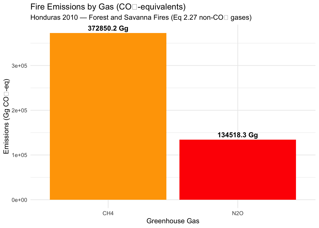
4.8 Uncertainty Analysis
4.8.1 Sources of Uncertainty
1. Emission Factor Uncertainty (IPCC Table 2.5):
| Gas | Forest (%) | Savanna (%) | Organic Soil (%) |
|---|---|---|---|
| CO2 | ±6 | ±6 | ±0.5 |
| CH4 | ±30-40 | ±40 | ±95 |
| N2O | ±50-60 | ±50 | N/A |
Note: Forest CO2 emission factor uncertainty (±6%) is relevant for cross-checking. The total uncertainty in forest CO2 reporting is dominated by stock-change uncertainty (biomass estimates, allometric models), not Gef.
2. Cumulative Uncertainty (from all chapters):
Recall from Chapter 3: \[ U_{total}^2 = U_A^2 + U_{MB}^2 + U_{Cf}^2 + U_{Gef}^2 \]
For Forest CH4 emissions:
- \(U_A\) = ±30% (burned area)
- \(U_{MB}\) = ±50% (fuel load)
- \(U_{Cf}\) = ±25% (combustion factor)
- \(U_{Gef}\) = ±35% (CH4 emission factor)
Combined uncertainty: \[ U_{total} = \sqrt{30^2 + 50^2 + 25^2 + 35^2} = \sqrt{4650} \approx 68\% \]
For Savanna emissions: ~85% uncertainty
For Organic soil CO2: ~60% uncertainty (dominated by fuel consumption)
4.8.2 Monte Carlo Uncertainty Propagation
# Parameters: Honduras Humid Tropical Forest
n_simulations <- 10000

# Mean values (from Ch1-3 GEE results)
MB_mean <- 119.6    # t DM ha⁻¹ (humid tropical)
Cf_mean <- 0.36
EF_CH4_mean <- 6.8  # g kg⁻¹ (tropical forest)

# Uncertainties (SD = 95% CI / 1.96)
MB_sd <- 52.4 / 1.96
Cf_sd <- 0.09 / 1.96
EF_CH4_sd <- 2.0 / 1.96

# Generate random samples (area fixed from GEE)
set.seed(42)
simulations <- data.frame(
  MB = rnorm(n_simulations, MB_mean, MB_sd),
  Cf = rnorm(n_simulations, Cf_mean, Cf_sd),
  EF_CH4 = rnorm(n_simulations, EF_CH4_mean, EF_CH4_sd)
) %>%
  mutate(
    MB = pmax(0, MB),
    Cf = pmin(1, pmax(0, Cf)),
    EF_CH4 = pmax(0, EF_CH4),
    # MB_Cf = fuel consumed (t DM ha⁻¹)
    # Emissions per ha = MB × Cf × EF × 10⁻³ (kg CH₄ ha⁻¹)
    CH4_kg_per_ha = MB * Cf * EF_CH4,
    # Relative to central estimate
    ratio = CH4_kg_per_ha / (MB_mean * Cf_mean * EF_CH4_mean)
  )

# Summary statistics
ratio_mean <- mean(simulations$ratio)
ratio_ci_lower <- quantile(simulations$ratio, 0.025)
ratio_ci_upper <- quantile(simulations$ratio, 0.975)

cat(sprintf("Honduras HTF CH₄ — Relative uncertainty\n"))
## Honduras HTF CH₄ — Relative uncertainty
cat(sprintf("  Mean ratio: %.2f\n", ratio_mean))
##   Mean ratio: 1.00
cat(sprintf("  95%% CI:    [%.2f, %.2f]\n",
            ratio_ci_lower, ratio_ci_upper))
##   95% CI:    [0.48, 1.66]
cat(sprintf("  i.e. -%d%% to +%d%% around central estimate\n",
            round((1 - ratio_ci_lower) * 100),
            round((ratio_ci_upper - 1) * 100)))
##   i.e. -52% to +66% around central estimate

# Visualize distribution
ggplot(simulations, aes(x = CH4_kg_per_ha)) +
  geom_histogram(bins = 50, fill = "steelblue", alpha = 0.7) +
  geom_vline(xintercept = MB_mean * Cf_mean * EF_CH4_mean,
             color = "red", linewidth = 1, linetype = "dashed") +
  labs(
    title = "Uncertainty Distribution: Tropical Forest CH₄ Emissions",
    subtitle = "Honduras — Monte Carlo (10,000 simulations)",
    x = "CH₄ Emissions (kg per ha burned)",
    y = "Frequency"
  ) +
  theme_minimal()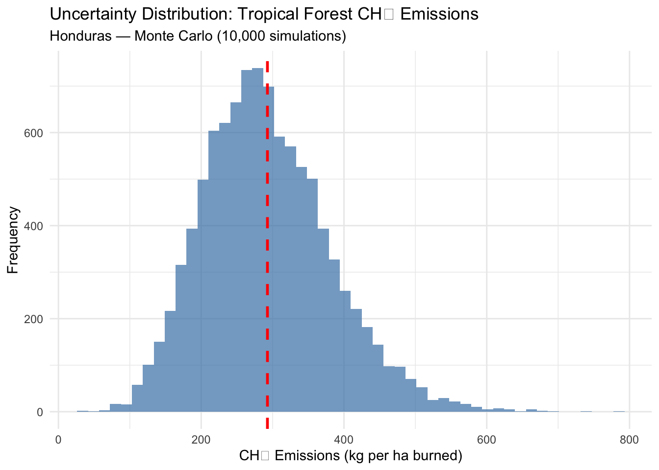
4.9 Spatial Emissions Mapping in GEE
4.9.1 Pixel-Level Emissions Calculation
# 1. Derive Emission Factor Rasters (non-CO₂ gases via Eq 2.27)
# CH₄ emission factors by vegetation type
EF_CH4_img <- ee$Image(0)$rename("EF_CH4")
EF_CH4_img <- EF_CH4_img$
  where(forest_mask$And(tropical), 6.8)$
  where(forest_mask$And(tropical$Not()), 4.7)$
  where(savanna_mask, 2.3)

# N₂O emission factors
EF_N2O_img <- ee$Image(0)$rename("EF_N2O")
EF_N2O_img <- EF_N2O_img$
  where(forest_mask$And(tropical), 0.20)$
  where(forest_mask$And(tropical$Not()), 0.26)$
  where(savanna_mask, 0.21)

# CO₂ emission factor raster (cross-check for forest only)
EF_CO2_img <- ee$Image(0)$rename("EF_CO2")
EF_CO2_img <- EF_CO2_img$
  where(forest_mask$And(tropical), 1580)$
  where(forest_mask$And(tropical$Not()), 1569)

# 2. Calculate Emissions Per Pixel
# CH₄ emissions (kg): biomass (t) × 1000 (kg/t) × EF (g/kg) / 1000 (g→kg)
CH4_per_pixel <- biomass_per_pixel$
  multiply(EF_CH4_img)$
  rename("CH4_kg")$
  clip(aoi_country_ee$geometry())

# N₂O emissions (kg)
N2O_per_pixel <- biomass_per_pixel$
  multiply(EF_N2O_img)$
  rename("N2O_kg")$
  clip(aoi_country_ee$geometry())

# CO₂ cross-check (forest only, kg)
CO2_crosscheck_per_pixel <- biomass_per_pixel$
  updateMask(forest_mask)$
  multiply(EF_CO2_img)$
  rename("CO2_crosscheck_kg")$
  clip(aoi_country_ee$geometry())

# 3. Visualize
ch4_vis <- list(
  min = 0L, max = 50L,
  palette = c("yellow", "orange", "red", "darkred")
)
n2o_vis <- list(
  min = 0L, max = 5L,
  palette = c("lightblue", "blue", "darkblue", "purple")
)

tmap::tmap_mode("view")
tmap::tm_shape(aoi_country_sf) + tmap::tm_borders(col = "white", lwd = 1.5) +
  tmap::tm_tiles(
    ee_tile_url(CH4_per_pixel$selfMask(), ch4_vis),
    group = "CH₄ Emissions (kg per pixel)"
  ) +
  tmap::tm_tiles(
    ee_tile_url(N2O_per_pixel$selfMask(), n2o_vis),
    group = "N₂O Emissions (kg per pixel)"
  ) +
  tmap::tm_add_legend(
    type = "polygons",
    fill = c("orange", "red", "blue", "purple"),
    labels = c("CH₄ Low", "CH₄ High", "N₂O Low", "N₂O High"),
    title = "GHG Emissions (kg/pixel)"
  ) +
  tmap::tm_scalebar(position = c("RIGHT", "BOTTOM"), text.size = 0.5) +
  tmap::tm_basemap("Esri.WorldImagery")
# Total CH₄ emissions
CH4_total <- CH4_per_pixel$
reduceRegion(
reducer = ee$Reducer$sum(),
geometry = aoi_country_ee$geometry(),
scale = 500L,
maxPixels = 1e9
)$getInfo()
# Total N₂O emissions
N2O_total <- N2O_per_pixel$
reduceRegion(
reducer = ee$Reducer$sum(),
geometry = aoi_country_ee$geometry(),
scale = 500L,
maxPixels = 1e9
)$getInfo()
# CO₂ cross-check (forest only)
CO2_crosscheck_total <- CO2_crosscheck_per_pixel$
reduceRegion(
reducer = ee$Reducer$sum(),
geometry = aoi_country_ee$geometry(),
scale = 500L,
maxPixels = 1e9
)$getInfo()
CH4_Gg <- (CH4_total[["CH4_kg"]] %||% 0) / 1e6
N2O_Gg <- (N2O_total[["N2O_kg"]] %||% 0) / 1e6
CO2_xcheck_Gg <- (CO2_crosscheck_total[["CO2_crosscheck_kg"]] %||% 0) / 1e6
cat("Honduras 2010 — GEE Pixel-Level Emissions\n")
## Honduras 2010 — GEE Pixel-Level Emissions
cat(" Total CH₄:", round(CH4_Gg, 4), "Gg\n")
## Total CH₄: 13.3 Gg
cat(" Total N₂O:", round(N2O_Gg, 5), "Gg\n")
## Total N₂O: 0.508 Gg
cat(" CH₄ CO₂-eq:", round(CH4_Gg * 28, 2), "Gg\n")
## CH₄ CO₂-eq: 372 Gg
cat(" N₂O CO₂-eq:", round(N2O_Gg * 265, 2), "Gg\n")
## N₂O CO₂-eq: 135 Gg
cat(" Total CO₂-eq (non-CO₂):",
round(CH4_Gg * 28 + N2O_Gg * 265, 2), "Gg\n")
## Total CO₂-eq (non-CO₂): 507 Gg
cat("\n Forest CO₂ cross-check:",
round(CO2_xcheck_Gg, 2), "Gg\n")
##
## Forest CO₂ cross-check: 2659 Gg
cat(" (Reported via stock changes, not fire emissions table)\n")
## (Reported via stock changes, not fire emissions table)4.10 NGHGI Reporting Format
4.10.1 IPCC Common Reporting Format (CRF)
Required tables for fire emissions:
- Table 4.C - Fires on Forest Land
- Area burned (ha)
- Biomass burned (tonnes DM)
- CH4 emissions (Gg)
- N2O emissions (Gg)
- Note: CO2 from forest fires is reported in the carbon stock change rows of Table 4.A, not here
- Table 4.F - Fires on Grassland
- Area burned (ha)
- Biomass burned (tonnes DM)
- CH4 emissions (Gg)
- N2O emissions (Gg)
- CO2: Not reported (Tier 1 synchrony assumption)
- Table 4(V) - Fires in Organic Soils (Wetlands Supplement)
- Area burned (ha)
- CO2 emissions (Gg)
- CH4 emissions (Gg)
# Format for CRF Table 4.C (Forest Land)
crf_4c <- emissions %>%
  filter(fire_category == "Forest") %>%
  group_by(country, year) %>%
  summarise(
    biomass_burned_t = sum(biomass_burned_Gg) * 1000,
    CH4_Gg = sum(emissions_Gg[gas == "CH4"]),
    N2O_Gg = sum(emissions_Gg[gas == "N2O"]),
    .groups = "drop"
  ) %>%
  mutate(
    IPCC_Category = "4.C.1",
    Subcategory = "Fires - Forest Land",
    Tier = "Tier 1",
    CO2_note = "CO₂ reported via stock changes (Table 4.A)"
  )

# Format for CRF Table 4.F (Grassland)
crf_4f <- emissions %>%
  filter(fire_category == "Savanna") %>%
  group_by(country, year) %>%
  summarise(
    biomass_burned_t = sum(biomass_burned_Gg) * 1000,
    CH4_Gg = sum(emissions_Gg[gas == "CH4"]),
    N2O_Gg = sum(emissions_Gg[gas == "N2O"]),
    .groups = "drop"
  ) %>%
  mutate(
    IPCC_Category = "4.F.1",
    Subcategory = "Fires - Grassland",
    Tier = "Tier 1",
    CO2_note = "CO₂ excluded (Tier 1 synchrony assumption)"
  )

# Combine for full CRF submission
crf_fires <- bind_rows(crf_4c, crf_4f)

# Export
write.csv(
  crf_fires,
  "Honduras_2010_CRF_Fires.csv",
  row.names = FALSE
)

library(knitr)
kable(
  crf_fires %>%
    select(IPCC_Category, Subcategory, biomass_burned_t,
           CH4_Gg, N2O_Gg, Tier, CO2_note),
  caption = "UNFCCC CRF Tables 4.C and 4.F — Honduras 2010 Fire Emissions",
  digits = c(0, 0, 0, 4, 5, 0, 0)
)| IPCC_Category | Subcategory | biomass_burned_t | CH4_Gg | N2O_Gg | Tier | CO2_note |
|---|---|---|---|---|---|---|
| 4.C.1 | Fires - Forest Land | 3365412 | 11442 | 337 | Tier 1 | CO₂ reported via stock changes (Table 4.A) |
| 4.F.1 | Fires - Grassland | 1629285 | 1874 | 171 | Tier 1 | CO₂ excluded (Tier 1 synchrony assumption) |
4.10.2 Documentation Requirements
IPCC Good Practice Guidance requires documentation of:
- Data sources:
- MODIS MCD64A1 Collection 6.1 (burned area)
- MODIS MCD12Q1 Collection 6.1 (land cover)
- IPCC 2019 Refinement Tables 2.4 and 2.5
- Methods:
- Tier 1 approach
- Equation 2.27 for non-CO2 gases
- Carbon stock changes (Eq. 2.7–2.14) for forest CO2
- Quality filters applied (uncertainty < 20%)
- CO2 accounting:
- Forest: CO2 reported through stock changes (2006 GL §4.2.4)
- Savanna: CO2 excluded per Tier 1 synchrony assumption (2019 Ref §2.4)
- Organic soils: CO2 reported separately (2013 WS Ch. 2)
- Uncertainty:
- Combined uncertainty: ±65-100%
- Major contributors: Fuel loads, combustion factors
- Monte Carlo analysis performed
- QA/QC procedures:
- Multi-source validation (GLAD, ESRI)
- Time series consistency checks
- Comparison with independent estimates
- Recalculations:
- If methodology changes: Recalculate entire time series
- Document changes in National Inventory Report (NIR)
4.11 Notes and Next Steps
4.11.1 Key Takeaways
- Emission factors convert biomass burned to gas emissions:
- CH4: 2.3-6.8 g kg-1 (savanna < forest)
- N2O: 0.20-0.26 g kg-1 (similar across types)
- CO2: 1580-1613 g kg-1 (forest/savanna, Table 2.5)
- CO2: 1703 g kg-1 (organic soils, Wetlands Supp.)
- CO2 reporting:
- Forest: CO2 is reported via carbon stock changes (not the fire emissions table); synchrony cannot be assumed for woody biomass (2006 GL §4.2.4)
- Savanna: CO2 excluded at Tier 1 (synchrony assumed for non-woody grassland), with caveats for woody systems (2019 Ref §2.4)
- Organic soils: CO2 reported directly (permanent carbon loss)
- CO2-equivalents:
- GWPCH4 = 28, GWPN2O = 265 (IPCC AR5)
- Total warming impact dominated by CH4 (65-70%)
- Uncertainty:
- Forest fires: ±68%
- Savanna fires: ±85%
- Driven by fuel consumption more than emission factors
- Reporting:
- UNFCCC CRF Tables 4.C (Forest) and 4.F (Grassland)
- Forest CO2 in stock change tables (4.A)
- Transparency documentation required
4.11.2 Chapter 5
Chapter 5: Organic Soils and Peatland Fires will expand on:
- Detailed peat fire methodology (IPCC Wetlands Supplement)
- Southeast Asia case studies (Indonesia, Malaysia)
- Drainage impacts on fire risk and emissions
- Depth of burn estimation techniques
- Smoldering combustion characteristics
Alternative pathway: If organic soils are not relevant to your region, Chapter 5 could cover:
- Quality control and validation procedures
- Time series analysis and trend detection
- Inter-annual variability and climate drivers
-
To confirm values, paged links to GWP values from AR5 here, AR2 here, and
AR6 here.AR6 states: “Under the Paris Rulebook [Decision 18/CMA.1, annex, paragraph 37], parties have agreed to use GWP100 values from the IPCC AR5 or GWP100 values from a subsequent IPCC Assessment Report to reportaggregate emissions and removals of GHGs. In addition, parties may use other metrics to report supplemental information on aggregate emissions and removals of GHGs.”↩︎