easypackages::packages(
  "bslib",
  "cols4all", "covr", "cowplot",
  "dendextend", "digest","DiagrammeR","dtwclust", "downlit",
  "e1071", "exactextractr","elevatr",
  "FNN", "future", "forestdata",
  "gdalcubes", "gdalUtilities", "geojsonsf", "geos", "ggplot2", "ggstats",
  "ggspatial", "ggmap", "ggplotify", "ggpubr", "ggrepel", "giscoR",
  "hdf5r", "httr", "httr2", "htmltools",
  "jsonlite",
  "kohonen", "knitr",
  "leaflet.providers", "leafem", "libgeos","luz","lwgeom", "leaflet", "leafgl",
  "mapedit", "mapview", "maptiles", "methods", "mgcv",
  "ncdf4", "nnet",
  "openxlsx", "parallel", "plotly",
  "randomForest", "rasterVis", "raster", "Rcpp", "RcppArmadillo",
  "RcppCensSpatial","rayshader", "RcppEigen", "RcppParallel",
  "RColorBrewer", "reactable", "rgl", "rsconnect","RStoolbox", "rts", "reticulate",
  "s2", "sf", "scales", "sits","spdep", "stars", "stringr","supercells",
  "terra", "testthat", "tidyverse", "tidyterra","tools",
  "tmap", "tmaptools", "terrainr",
  "xgboost",
  prompt = F)

#mapviewOptions(fgb = FALSE)
sf::sf_use_s2(use_s2 = FALSE)3 Fuel Consumption
Overview
This chapter describes the estimation of fuel mass available for combustion (MB) and combustion factors (Cf) following IPCC Tier 1 default values. These parameters, combined with burned area and vegetation classifications from Chapters 1-2, determine the total biomass burned in fire events.
Environment Setup
IPCC Fuel Biomass
3.0.1 Component in Equation 2.27
Fuel biomass consumption represents two components of the IPCC fire emissions equation:
\[ L_{fire} = A \times M_B \times C_f \times G_{ef} \times 10^{-3} \]
Where: - MB = Mass of fuel available for combustion (tonnes dry matter ha⁻¹) - Cf = Combustion factor (dimensionless, 0-1) - MB × Cf = Actual biomass consumed per unit area (tonnes DM ha⁻¹)
Tier 1 Approach: Use IPCC default values stratified by:
- Vegetation type (Forest, Savanna, Organic Soil)
- Climate zone (Tropical, Temperate, Boreal)
- Forest type (Humid Tropical vs. Other)
- Season (Early vs. Late dry season for savannas)
3.0.2 IPCC Default Values - Quick Reference
Forest Fires (IPCC 2019 Table 2.4):
| Forest Type | MB (t DM ha⁻¹) | Cf | MB × Cf |
|---|---|---|---|
| Humid Tropical Forest | 119.6 ± 52.4 | 0.36 ± 0.09 | 43.1 |
| Other Forest (Boreal) | 41.0 ± 25.3 | 0.45 ± 0.15 | 18.5 |
| Other Forest (Temperate) | 50.4 ± 30.8 | 0.47 ± 0.14 | 23.7 |
| Other Forest (Tropical) | 69.4 ± 44.3 | 0.47 ± 0.14 | 32.6 |
Savanna Fires (IPCC 2019 Table 2.4):
| Vegetation Type | Season | MB (t DM ha⁻¹) | Cf | MB × Cf |
|---|---|---|---|---|
| Savanna Woodland | Early | 9.0 ± 7.5 | 0.29 ± 0.09 | 2.6 |
| Savanna Woodland | Late | 9.0 ± 7.5 | 0.51 ± 0.15 | 4.6 |
| Savanna Grassland | Early | 6.8 ± 6.0 | 0.31 ± 0.09 | 2.1 |
| Savanna Grassland | Late | 6.8 ± 6.0 | 0.83 ± 0.15 | 5.6 |
| Other Grassland | - | 13.4 ± 8.8 | 0.52 ± 0.15 | 7.0 |
Organic Soil Fires (IPCC 2014 Wetlands Supplement Table 2.6):
| Soil Type | MB (t DM ha⁻¹) | Cf | MB × Cf |
|---|---|---|---|
| Tropical Peatland | 41.2 ± 1.4 | 1.0 | 41.2 |
Note: Organic soil combustion factor = 1.0 assumes complete consumption of affected layer.
3.1 Fuel Available for Combustion (MB)
3.1.1 Forest Fuel Loads
3.1.1.1 Components of Forest Fuel
Forest fuel includes multiple strata burned during fire:
Surface Fuels:
- Litter (freshly fallen leaves, needles)
- Duff (decomposed organic layer)
- Herbaceous vegetation
- Woody debris (< 7.5 cm diameter)
Ground Fuels:
- Organic soil horizons (O and A)
- Roots (fine and coarse)
- Stumps and buried wood
Crown Fuels (stand-replacing fires only):
- Foliage
- Fine branches
- Bark
- Lichen and epiphytes
Tier 1 Simplification: MB represents average fuel consumed across fire severity gradient, from surface fires (low MB) to crown fires (high MB).
3.1.1.2 Climate-Dependent Forest Fuel Loads
Boreal Forests (41.0 t DM ha⁻¹):
- Slow decomposition
- thick organic layers
- Coniferous litter high in lignin
- Permafrost limits root depth
- Fire-adapted species (e.g., Pinus sylvestris)
Temperate Forests (50.4 t DM ha⁻¹):
- Moderate decomposition rates
- Mixed deciduous/coniferous litter
- Seasonal accumulation patterns
- Variable fire regimes
Tropical Forests (69.4 t DM ha⁻¹):
- Rapid decomposition → less litter, but high biomass density
- Fire-sensitive under natural conditions
- Droughts enable fire spread
Humid Tropical Forests (119.6 t DM ha⁻¹):
- Highest fuel loads due to:
- Dense canopy biomass
- Multi-story structure
- Epiphytes, vines, and bamboo
- Deep root systems
- Primarily deforestation fires (slash-and-burn)
- Stand-replacing events
3.1.2 Savanna Fuel Loads
3.1.2.1 Savanna Fuel Characteristics
Dominant fuel type: Herbaceous grass (70-90% of fuel consumed)
Key determinants of fuel load:
- Annual precipitation: Grass productivity increases with rainfall
- Season: Fuel cures (dries) during dry season
- Fire frequency: Frequent fires -> lower woody component
- Grazing pressure: Reduces available fuel
Spatial heterogeneity: Fuel patchy due to:
- Termite mounds (fuel-free zones)
- Tree shade (reduced grass growth)
- Grazing concentration around water
- Previous fire scars
3.1.2.2 Climate-Dependent Savanna Fuel Loads
Tropical Savannas (500-1500 mm rainfall):
- High grass productivity
- Distinct wet/dry seasons
- Fuel curing rapid
- MB: 6.8-9.0 t DM ha⁻¹
Temperate Grasslands (250-750 mm rainfall):
- Lower productivity than tropical
- Variable seasonality
- Mixed grass/forb composition
- MB: 13.4 t DM ha⁻¹ (includes crop residues)
Woody Savannas vs. Open Savannas:
- Woody component adds coarse fuels, but canopy reduces grass fuel
- Net effect: Similar MB to open savanna
- Combustion factor varies more than fuel load
3.1.2.3 Seasonal Dynamics
Early Dry Season:
- Fuel partially cured (50-70% dry matter)
- Lower combustion efficiency
- Lower Cf: 0.29-0.31
- Total consumption: 2.1-2.6 t DM ha⁻¹
Late Dry Season:
- Fuel fully cured (>90% dry matter)
- Complete combustion of grass layer
- Higher Cf: 0.51-0.83
- Total consumption: 4.6-5.6 t DM ha⁻¹
3.1.3 Organic Soil Fuel Loads
3.1.3.1 Peat Fuel Characteristics
Definition: Organic soils (Histosols) with >30 cm organic layer
Fuel properties:
- High carbon content: 50-60% C by dry weight
- Variable bulk density: 0.05-0.20 g cm⁻³
- High moisture retention: 200-1000% (dry weight basis)
- Smoldering combustion: Can burn for months
Fire behavior:
- Surface fires: Consume litter and upper peat (10-30 cm)
- Deep burns: Consume entire peat layer to mineral soil (>100 cm)
- Drainage amplifies risk: Drained peat extremely flammable
3.1.3.2 Fuel Load Calculation
IPCC Wetlands Supplement Approach:
\[ M_B = D_{burn} \times BD \times 10 \]
Where:
- \(D_{burn}\) = Depth of burn (cm)
- \(BD\) = Bulk density of peat (g cm⁻³)
- 10 = Conversion factor (cm = m, g cm⁻³ = t ha⁻¹)
IPCC Default (Southeast Asia):
- Depth of burn: 41 cm (range: 18-65 cm)
- Bulk density: 0.10 g cm⁻³ (range: 0.05-0.15)
- MB: 41.2 t DM ha⁻¹
High uncertainty: Coefficient of variation ~50%
3.2 Combustion Factor (Cf)
3.2.1 Definition and Interpretation
Combustion Factor (Cf) = Proportion of available fuel actually consumed by fire
\[ C_f = \frac{\text{Mass of fuel consumed}}{\text{Mass of fuel available}} \quad (0 \leq C_f \leq 1) \]
Determinants:
- Fuel moisture: Higher moisture = lower Cf
- Fire intensity: Hotter fires → higher Cf
- Fire type: Surface vs. crown fire
- Fuel particle size: Fine fuels (< 0.6 cm) burn more completely
- Weather conditions: Wind, humidity, temperature
3.2.2 Forest Combustion Factors
Low Cf for Humid Tropical Forests (0.36):
- High ambient moisture
- Rapid fuel accumulation = green fuels mixed with dead
- Incomplete combustion of large woody debris
- Char and partially burned material remain
Moderate Cf for Other Forests (0.45-0.47):
- Drier climates = lower fuel moisture
- More complete consumption of surface fuels
- Variability based on fire severity:
- Surface fires: Cf ~ 0.20-0.40
- Crown fires: Cf ~ 0.60-0.80
- Default represents average across severities
3.2.3 Savanna Combustion Factors
Early Dry Season (0.29-0.31):
- Fuel partially cured
- High moisture content in live grass (30-50%)
- Incomplete combustion - Patchy fire spread
- Much grass left standing
Late Dry Season (0.51-0.83):
- Fuel fully cured (<10% moisture)
- Complete consumption of grass layer
- Only woody stems and char remain
- Higher Cf for grasslands vs. woody savannas:
- Grassland: Cf = 0.83 (almost complete)
- Woody Savanna: Cf = 0.51 (trees create shade/barriers)
Physical explanation: \[ C_f \propto \frac{1}{\text{Fuel Moisture}} \times \text{Fire Intensity} \]
Late season = Lower moisture × Higher intensity = Higher Cf
3.2.4 Organic Soil Combustion Factors
Complete Consumption (Cf = 1.0):
- Once peat ignites, burns to completion within affected depth
- Smoldering combustion eliminates unburned fuel
- Char production minimal
- Caveat: Cf = 1.0 applies to depth of burn, not total peat column
- If burn depth = 41 cm, that 41 cm is fully consumed
- Deeper peat layers remain intact (if fire extinguished)
3.3 Applying Fuel Consumption Parameters
3.3.1 Workflow: Vegetation Type to Fuel Values
library(tidyverse)

# IPCC 2019 Table 2.4 - Default fuel consumption values
fuel_consumption_table <- tribble(
  ~fire_category, ~vegetation_type, ~climate_zone, ~season, ~MB_tDM_ha, ~Cf, ~MB_Cf,

  # Forest Fires
  "Forest", "Humid_Tropical_Forest", "Tropical_Moist", NA, 119.6, 0.36, 43.1,
  "Forest", "Other_Forest", "Boreal", NA, 41.0, 0.45, 18.5,
  "Forest", "Other_Forest", "Temperate", NA, 50.4, 0.47, 23.7,
  "Forest", "Other_Forest", "Tropical", NA, 69.4, 0.47, 32.6,

  # Savanna Fires
  "Savanna", "Savanna_Woodland", "All", "Early", 9.0, 0.29, 2.6,
  "Savanna", "Savanna_Woodland", "All", "Late", 9.0, 0.51, 4.6,
  "Savanna", "Savanna_Grassland", "All", "Early", 6.8, 0.31, 2.1,
  "Savanna", "Savanna_Grassland", "All", "Late", 6.8, 0.83, 5.6,
  "Savanna", "Other_Grassland", "All", NA, 13.4, 0.52, 7.0,

  # Organic Soil Fires
  "Organic_Soil", "Tropical_Peatland", "Tropical", NA, 41.2, 1.0, 41.2
)

print(fuel_consumption_table)
## # A tibble: 10 × 7
##   fire_category vegetation_type       climate_zone   season
##   <chr>         <chr>                 <chr>          <chr>
## 1 Forest        Humid_Tropical_Forest Tropical_Moist <NA>
## 2 Forest        Other_Forest          Boreal         <NA>
## 3 Forest        Other_Forest          Temperate      <NA>
## 4 Forest        Other_Forest          Tropical       <NA>
## 5 Savanna       Savanna_Woodland      All            Early
## 6 Savanna       Savanna_Woodland      All            Late
## # ℹ 4 more rows
## # ℹ 3 more variables: MB_tDM_ha <dbl>, Cf <dbl>,
## #   MB_Cf <dbl>

# Save for use in emissions calculation
write.csv(
  fuel_consumption_table,
  "IPCC_fuel_consumption_defaults.csv",
  row.names = FALSE
)
3.4 GEE Initialisation
# Point environment to your configured python
reticulate::use_python("/opt/local/bin/python", required=T)

# Initialise Earth Engine
ee <- reticulate::import("ee")
ee$Initialize(project = "murphys-deforisk")
cat("GEE initialised\n")
## GEE initialised

# Helper: visualize EE tile in tmap/leaflet
ee_tile_url <- function(ee_image, vis_params) {
  ee_image$getMapId(vis_params)$tile_fetcher$url_format
}

# Helper: EE FeatureCollection => sf
ee_to_sf <- function(fc) {
  geojsonsf::geojson_sf(
    jsonlite::toJSON(fc$getInfo(), auto_unbox = TRUE))
}

# Load AOI boundaries from FAO GAUL
aoi_country_ee <- ee$FeatureCollection("FAO/GAUL/2015/level0")$
  filter(ee$Filter$eq("ADM0_NAME", "Honduras"))
aoi_states_ee  <- ee$FeatureCollection("FAO/GAUL/2015/level1")$
  filter(ee$Filter$eq("ADM0_NAME", "Honduras"))
aoi_country_sf <- ee_to_sf(aoi_country_ee)
aoi_states_sf  <- ee_to_sf(aoi_states_ee)

cat("AOI loaded:", aoi_country_ee$size()$getInfo(), "country,",
    aoi_states_ee$size()$getInfo(), "states\n")
## AOI loaded: 1 country, 19 states
3.4.1 Upstream Inputs from Chapters 1-2
# --- Chapter 1: Burned area (MCD64A1) ---
mcd64 <- ee$ImageCollection("MODIS/061/MCD64A1")
burned_2010 <- mcd64$
  filterBounds(aoi_country_ee$geometry())$
  filterDate("2010-01-01", "2010-12-31")

# FAOSTAT quality filter (matching Ch1)
faostat_filter <- function(image) {
  unc  <- image$select("Uncertainty")
  burn <- image$select("BurnDate")
  mask <- unc$lt(20L)$And(burn$gt(0L))
  image$updateMask(mask)
}

# Annual burned mask for 2010
annual_burned_2010 <- burned_2010$
  map(faostat_filter)$
  select("BurnDate")$max()$gt(0L)$selfMask()

# --- Chapter 2: Land cover & vegetation masks ---
lc_2010 <- ee$ImageCollection("MODIS/061/MCD12Q1")$
  select("LC_Type1")$
  filterDate("2010-01-01", "2010-12-31")$
  first()$
  clip(aoi_country_ee$geometry())

# Forest mask (IGBP 1-5)
forest_mask <- lc_2010$gte(1L)$And(lc_2010$lte(5L))

# Savanna/grassland mask (IGBP 6-10)
savanna_mask <- lc_2010$gte(6L)$And(lc_2010$lte(10L))

# Climate-based humid tropical delineation
bio <- ee$Image("WORLDCLIM/V1/BIO")
precip <- bio$select("bio12")
temp   <- bio$select("bio01")

tropical <- temp$gt(180L)
moist    <- precip$gt(1500L)
humid_tropical_mask <- tropical$And(moist)

# Forest sub-types
humid_tropical_forest <- forest_mask$And(humid_tropical_mask)
other_forest          <- forest_mask$And(humid_tropical_mask$Not())

# Pixel area helper
pixelArea_ha <- ee$Image$pixelArea()$divide(10000L)

cat("Upstream inputs loaded: MCD64A1 + MCD12Q1 + WorldClim\n")
## Upstream inputs loaded: MCD64A1 + MCD12Q1 + WorldClim
3.5 Spatial Implementation in Google Earth Engine
3.5.1 Creating Fuel Consumption Rasters
# Climate zone masks
boreal    <- temp$lt(0L)
temperate <- temp$gte(0L)$And(temp$lte(180L))

# Create fuel consumption image (M_B × C_f in t DM ha⁻¹)
fuel_consumption <- ee$Image(0)$rename("fuel_consumption")

# 1. Humid Tropical Forest (M_B × C_f = 43.1)
htf_mask <- forest_mask$And(humid_tropical_mask)
fuel_consumption <- fuel_consumption$where(htf_mask, 43.1)

# 2. Other Forest - Boreal (M_B × C_f = 18.5)
forest_boreal <- forest_mask$And(boreal)$And(humid_tropical_mask$Not())
fuel_consumption <- fuel_consumption$where(forest_boreal, 18.5)

# 3. Other Forest - Temperate (M_B × C_f = 23.7)
forest_temperate <- forest_mask$And(temperate)$And(humid_tropical_mask$Not())
fuel_consumption <- fuel_consumption$where(forest_temperate, 23.7)

# 4. Other Forest - Tropical Dry (M_B × C_f = 32.6)
forest_tropical <- forest_mask$And(tropical)$And(humid_tropical_mask$Not())
fuel_consumption <- fuel_consumption$where(forest_tropical, 32.6)

# 5. Savanna/Grassland (average = 7.0 t DM ha⁻¹)
fuel_consumption <- fuel_consumption$where(savanna_mask, 7.0)

# Apply to burned areas only
fuel_burned <- fuel_consumption$
  updateMask(annual_burned_2010)$
  clip(aoi_country_ee$geometry())

# Visualize
fuel_vis <- list(
  min = 0L, max = 50L,
  palette = c("yellow", "orange", "red", "darkred")
)

tmap::tmap_mode("view")
tmap::tm_shape(aoi_country_sf) + tmap::tm_borders(col = "white", lwd = 1.5) +
  tmap::tm_tiles(
    ee_tile_url(fuel_burned, fuel_vis),
    group = "Fuel Consumption (t DM ha⁻¹)"
  ) +
  tmap::tm_add_legend(
    type = "polygons",
    fill = c("yellow", "orange", "red", "darkred"),
    labels = c("Savanna (~7)", "Temperate Forest (~24)",
               "Tropical Forest (~33)", "Humid Tropical (~43)"),
    title = "Fuel Consumption (t DM ha⁻¹)"
  ) +
  tmap::tm_scalebar(position = c("RIGHT", "BOTTOM"), text.size = 0.5) +
  tmap::tm_basemap("Esri.WorldImagery")
3.5.2 Seasonal Stratification for Savannas
# Extract burn month from MCD64A1
extractBurnMonth <- function(mcd64_image) {
  burn_date <- mcd64_image$select("BurnDate")
  img_date  <- ee$Date(mcd64_image$get("system:time_start"))
  month     <- img_date$get("month")

  month_band <- ee$Image$constant(month)$
    updateMask(burn_date$gt(0L))$
    rename("burn_month")$
    toInt()

  burn_date$addBands(month_band)
}

# Apply to 2010 collection (quality-filtered)
mcd64_with_months <- burned_2010$
  map(faostat_filter)$
  map(extractBurnMonth)

# Composite: latest month if pixel burned multiple times
month_composite <- mcd64_with_months$
  select("burn_month")$
  max()

# Honduras dry season (Central America)
# Early dry: Feb-Mar (months 2-3)
# Late dry:  Apr-May (months 4-5)
early_season <- month_composite$gte(2L)$And(month_composite$lte(3L))
late_season  <- month_composite$gte(4L)$And(month_composite$lte(5L))

# Savanna fire subsets
savanna_fires_2010 <- annual_burned_2010$updateMask(savanna_mask)

# Woody savanna (IGBP class 8)
woody_savanna <- lc_2010$eq(8L)
# Grassland/savanna (IGBP classes 9-10)
grassland <- lc_2010$gte(9L)$And(lc_2010$lte(10L))

# Create seasonal fuel consumption
fuel_seasonal <- ee$Image(0)$rename("fuel_seasonal")
fuel_seasonal <- fuel_seasonal$
  where(woody_savanna$And(early_season), 2.6)$
  where(woody_savanna$And(late_season), 4.6)$
  where(grassland$And(early_season), 2.1)$
  where(grassland$And(late_season), 5.6)

# Mask to burned savanna areas
fuel_seasonal_burned <- fuel_seasonal$
  updateMask(savanna_fires_2010)$
  clip(aoi_country_ee$geometry())

# Visualize
tmap::tm_shape(aoi_country_sf) + tmap::tm_borders(col = "white", lwd = 1.5) +
  tmap::tm_tiles(
    ee_tile_url(fuel_seasonal_burned,
      list(min = 0L, max = 6L,
           palette = c("lightyellow", "yellow", "orange"))),
    group = "Savanna Fuel Consumption (Seasonal)"
  ) +
  tmap::tm_add_legend(
    type = "polygons",
    fill = c("lightyellow", "yellow", "orange"),
    labels = c("Early grassland (2.1)", "Early woody (2.6) / Late woody (4.6)",
               "Late grassland (5.6)"),
    title = "Savanna Fuel (t DM ha⁻¹)"
  ) +
  tmap::tm_scalebar(position = c("RIGHT", "BOTTOM"), text.size = 0.5) +
  tmap::tm_basemap("Esri.WorldImagery")
3.5.3 Calculating Total Biomass Burned
# Biomass burned per pixel (t DM) = fuel_consumption (t ha⁻¹) × area (ha)
biomass_per_pixel <- fuel_burned$multiply(pixelArea_ha)

# Forest biomass
forest_biomass <- biomass_per_pixel$
  updateMask(forest_mask)$
  reduceRegion(
    reducer   = ee$Reducer$sum(),
    geometry  = aoi_country_ee$geometry(),
    scale     = 500L,
    maxPixels = 1e9
  )$getInfo()

# Savanna biomass
savanna_biomass <- biomass_per_pixel$
  updateMask(savanna_mask)$
  reduceRegion(
    reducer   = ee$Reducer$sum(),
    geometry  = aoi_country_ee$geometry(),
    scale     = 500L,
    maxPixels = 1e9
  )$getInfo()

forest_t  <- forest_biomass[["fuel_consumption"]] %||% 0
savanna_t <- savanna_biomass[["fuel_consumption"]] %||% 0

cat("Honduras 2010 — Total Biomass Burned\n")
## Honduras 2010 — Total Biomass Burned
cat("  Forest biomass burned: ", round(forest_t / 1000, 1), "Gg DM\n")
##   Forest biomass burned:  1683 Gg DM
cat("  Savanna biomass burned:", round(savanna_t / 1000, 1), "Gg DM\n")
##   Savanna biomass burned: 815 Gg DM
cat("  Total:                 ", round((forest_t + savanna_t) / 1000, 1), "Gg DM\n")
##   Total:                  2497 Gg DM
3.5.4 Matching Vegetation Classifications to Fuel Values
# Burned area by vegetation type (from Ch2 overlay)
htf_fires  <- annual_burned_2010$updateMask(humid_tropical_forest)
of_fires   <- annual_burned_2010$updateMask(other_forest)
sav_fires  <- annual_burned_2010$updateMask(savanna_mask)

# Calculate areas (ha)
htf_area <- htf_fires$multiply(pixelArea_ha)$reduceRegion(
  reducer = ee$Reducer$sum(), geometry = aoi_country_ee$geometry(),
  scale = 500L, maxPixels = 1e9)$getInfo()
of_area <- of_fires$multiply(pixelArea_ha)$reduceRegion(
  reducer = ee$Reducer$sum(), geometry = aoi_country_ee$geometry(),
  scale = 500L, maxPixels = 1e9)$getInfo()
sav_area <- sav_fires$multiply(pixelArea_ha)$reduceRegion(
  reducer = ee$Reducer$sum(), geometry = aoi_country_ee$geometry(),
  scale = 500L, maxPixels = 1e9)$getInfo()

htf_ha <- htf_area[["BurnDate"]] %||% 0
of_ha  <- of_area[["BurnDate"]] %||% 0
sav_ha <- sav_area[["BurnDate"]] %||% 0

# Apply IPCC default fuel consumption
honduras_fuel <- tribble(
  ~fire_category, ~vegetation_type, ~area_ha, ~MB_tDM_ha, ~Cf, ~MB_Cf,
  "Forest", "Humid_Tropical_Forest", round(htf_ha, 1), 119.6, 0.36, 43.1,
  "Forest", "Other_Forest",          round(of_ha, 1),  69.4, 0.47, 32.6,
  "Savanna", "Savanna_Mixed",        round(sav_ha, 1),  7.9, 0.46,  3.6
) %>%
  mutate(
    biomass_burned_tDM = area_ha * MB_Cf,
    biomass_burned_Gg  = biomass_burned_tDM / 1000
  )

print(honduras_fuel)
## # A tibble: 3 × 8
##   fire_category vegetation_type      area_ha MB_tDM_ha    Cf
##   <chr>         <chr>                  <dbl>     <dbl> <dbl>
## 1 Forest        Humid_Tropical_Fore…  33688.     120.   0.36
## 2 Forest        Other_Forest           7163.      69.4  0.47
## 3 Savanna       Savanna_Mixed        116378.       7.9  0.46
## # ℹ 3 more variables: MB_Cf <dbl>,
## #   biomass_burned_tDM <dbl>, biomass_burned_Gg <dbl>

cat("\nHonduras 2010 — Summary\n")
##
## Honduras 2010 — Summary
cat("  Total burned area:     ", sum(honduras_fuel$area_ha), "ha\n")
##   Total burned area:      157229 ha
cat("  Total biomass burned:  ", round(sum(honduras_fuel$biomass_burned_Gg), 1), "Gg DM\n")
##   Total biomass burned:   2104 Gg DM
3.6 Uncertainty in Fuel Consumption Estimates
3.6.1 Sources of Uncertainty
1. IPCC Default Value Uncertainty:
IPCC provides 95% confidence intervals for all default values:
| Parameter | Relative Uncertainty |
|---|---|
| MB (Forest) | ±40-60% |
| MB (Savanna) | ±60-90% |
| Cf (Forest) | ±20-30% |
| Cf (Savanna) | ±30-40% |
| MB×Cf (combined) | ±50-70% |
2. Spatial Extrapolation Uncertainty:
- IPCC values derived from limited field studies
- Geographic bias toward well-studied regions (North America, Australia)
- Under-representation of tropical systems
3. Fire Severity Variability:
- Default values represent averages across fire severity spectrum
- Individual fires may have 2-3× higher/lower consumption
- No severity stratification in Tier 1
4. Temporal Variability:
- Fuel accumulation varies with:
- Time since last fire
- Precipitation anomalies (ENSO, droughts)
- Forest management (fuel reduction treatments)
- Tier 1 assumes constant fuel loads
3.6.2 Quantifying Combined Uncertainty
Following IPCC Error Propagation (Chapter 3, Equation 3.1):
\[ U_{total}^2 = U_A^2 + U_{MB}^2 + U_{Cf}^2 + U_{Gef}^2 \]
For Tier 1 Forest Fires:
- \(U_A\) = ±30% (from Chapter 1 - burned area)
- \(U_{MB}\) = ±50% (IPCC Table 2.4)
- \(U_{Cf}\) = ±25% (IPCC Table 2.4)
- \(U_{Gef}\) = ±30% (Chapter 4 - emission factors)
Combined uncertainty (quadrature): \[ U_{total} = \sqrt{30^2 + 50^2 + 25^2 + 30^2} = \sqrt{4350} \approx 66\% \]
For Tier 1 Savanna Fires:
- \(U_A\) = ±30%
- \(U_{MB}\) = ±80% (higher variability)
- \(U_{Cf}\) = ±35%
- \(U_{Gef}\) = ±30%
Combined uncertainty: \[ U_{total} = \sqrt{30^2 + 80^2 + 35^2 + 30^2} = \sqrt{9925} \approx 100\% \]
Interpretation: Tier 1 uncertainties are large but expected given coarse default values. Tier 2/3 approaches reduce uncertainty through country-specific data.
3.6.3 Sensitivity Analysis
library(tidyverse)

# Define parameter ranges (from IPCC confidence intervals)
# Honduras is predominantly humid tropical forest
fuel_params <- expand.grid(
  MB_forest = c(119.6 - 52.4, 119.6, 119.6 + 52.4),
  Cf_forest = c(0.36 - 0.09, 0.36, 0.36 + 0.09),
  area_ha = round(htf_ha, 0)
)

# Calculate biomass burned for each parameter combination
fuel_params <- fuel_params %>%
  mutate(
    biomass_tDM = area_ha * MB_forest * Cf_forest,
    biomass_Gg = biomass_tDM / 1000,
    scenario = paste0("MB=", round(MB_forest, 1),
                      ", Cf=", round(Cf_forest, 2))
  )

# Visualize sensitivity
ggplot(fuel_params, aes(x = MB_forest, y = Cf_forest,
                        fill = biomass_Gg)) +
  geom_tile() +
  geom_text(aes(label = round(biomass_Gg, 0)),
            color = "white", fontface = "bold") +
  scale_fill_viridis_c(name = "Biomass\nBurned (Gg)") +
  labs(
    title = "Sensitivity of Biomass Burned to Fuel Parameters",
    subtitle = paste("Honduras Humid Tropical Forest Fires (",
                     round(htf_ha, 0), "ha)"),
    x = "Fuel Load MB (t DM ha⁻¹)",
    y = "Combustion Factor Cf"
  ) +
  theme_minimal()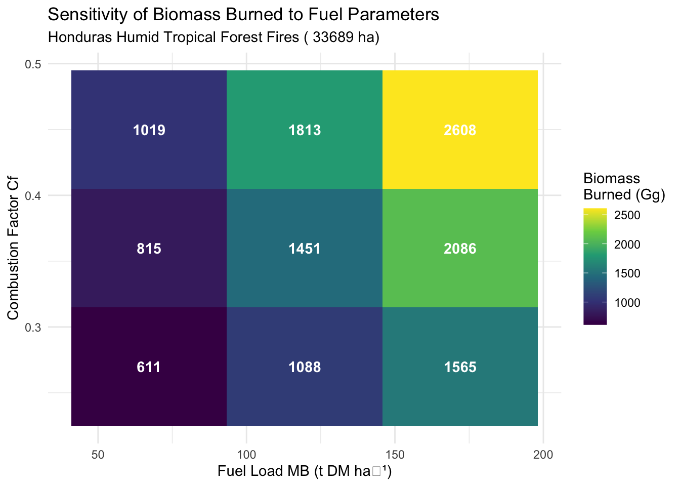
3.7 Advanced Topics
3.7.1 Country-Specific Fuel Data (Tier 2)
Moving beyond defaults:
When available, countries can use:
- National forest inventory data: Standing biomass, litter depths
- Fire behavior models: BEHAVE, FuelCalc, FCCS
- Field measurements: Post-fire fuel consumption studies
- Remote sensing: LiDAR for 3D fuel structure
Example: Honduras:
# Hypothetical: Honduras National Forest Inventory fuel loads
honduras_fuel_data <- tribble(
  ~forest_type, ~MB_tDM_ha, ~Cf, ~source,
  "Pinus caribaea (lowland pine)", 72.5, 0.42, "ICF National Inventory 2018",
  "Broadleaf humid forest",       125.3, 0.34, "SIGMOF field plots 2019",
  "Dry broadleaf / pine-oak",      55.8, 0.45, "La Mosquitia fire studies 2017"
)

# These values would replace IPCC defaults for Honduran forests
# Result: Reduced uncertainty (~±25% over ±50%)
print(honduras_fuel_data)
## # A tibble: 3 × 4
##   forest_type                   MB_tDM_ha    Cf source
##   <chr>                             <dbl> <dbl> <chr>
## 1 Pinus caribaea (lowland pine)      72.5  0.42 ICF Nationa…
## 2 Broadleaf humid forest            125.   0.34 SIGMOF fiel…
## 3 Dry broadleaf / pine-oak           55.8  0.45 La Mosquiti…
3.7.2 Tier 2+ Fire Severity Stratification (Pending)
Fire severity classes:
| Severity | dNBR Range | Cf Multiplier |
|---|---|---|
| Unburned | < 0.1 | 0 |
| Low | 0.1 - 0.27 | 0.5× |
| Moderate | 0.27 - 0.44 | 1.0× (default) |
| High | > 0.44 | 1.5× |
# Calculate dNBR from Landsat or Sentinel-2 to adjust Cf
# Pre-fire composite (Jan-Feb 2010)
prefire <- ee$ImageCollection("LANDSAT/LT05/C02/T1_L2")$
  filterBounds(aoi_country_ee$geometry())$
  filterDate("2010-01-01", "2010-02-28")$
  median()

# Post-fire composite (Jun-Jul 2010)
postfire <- ee$ImageCollection("LANDSAT/LT05/C02/T1_L2")$
  filterBounds(aoi_country_ee$geometry())$
  filterDate("2010-06-01", "2010-07-31")$
  median()

# Calculate NBR
calculateNBR <- function(img) {
  nir  <- img$select("SR_B4")
  swir <- img$select("SR_B7")
  nir$subtract(swir)$divide(nir$add(swir))$rename("NBR")
}
nbr_pre  <- calculateNBR(prefire)
nbr_post <- calculateNBR(postfire)
dnbr     <- nbr_pre$subtract(nbr_post)

# Define severity classes
low_severity      <- dnbr$gte(0.1)$And(dnbr$lt(0.27))
moderate_severity <- dnbr$gte(0.27)$And(dnbr$lt(0.44))
high_severity     <- dnbr$gte(0.44)

# Adjust combustion factor for humid tropical forest
Cf_default <- 0.36
Cf_adjusted <- ee$Image(Cf_default)$
  where(low_severity, Cf_default * 0.5)$
  where(high_severity, Cf_default * 1.5)

# Recalculate fuel consumption
MB <- 119.6
fuel_consumption_adjusted <- ee$Image(MB)$multiply(Cf_adjusted)
3.7.3 Fuel Moisture Effects
Fuel moisture reduces combustion efficiency:
\[ C_f = C_{f,dry} \times e^{-k \times MC} \]
Where:
- \(C_{f,dry}\) = Combustion factor at 0% moisture
- \(MC\) = Moisture content (%)
- \(k\) = Decay constant (~0.02 for grass, ~0.01 for wood)
# Load ERA5 relative humidity or precipitation data
precip_monthly <- ee$ImageCollection("ECMWF/ERA5/MONTHLY")$
  select("total_precipitation")

# Get precipitation in month of fire
# (Would need to match with burn dates from Chapter 1)

# For demonstration: use annual average
precip_annual <- precip_monthly$
  filterDate("2010-01-01", "2010-12-31")$
  mean()

# Convert to fuel moisture proxy (simplified)
# Assume: High precip → High moisture → Low Cf
# (Actual relationship requires mechanistic model)

# This is TIER 3 level - requires significant data and validation
3.8 Integrated Emissions Calculations
3.8.1 Output Formats
Required data structure:
# Create comprehensive fuel consumption table
fuel_output <- tribble(
  ~country, ~year, ~fire_category, ~vegetation_type, ~climate_zone, ~season,
  ~area_ha, ~MB_tDM_ha, ~Cf, ~biomass_burned_Gg,

  "Honduras", 2010, "Forest", "Humid_Tropical_Forest", "Tropical_Moist", NA,
  round(htf_ha, 0), 119.6, 0.36, round(htf_ha * 43.1 / 1000, 1),

  "Honduras", 2010, "Forest", "Other_Forest", "Tropical", NA,
  round(of_ha, 0), 69.4, 0.47, round(of_ha * 32.6 / 1000, 1),

  "Honduras", 2010, "Savanna", "Savanna_Mixed", "Tropical", "Late",
  round(sav_ha, 0), 7.9, 0.46, round(sav_ha * 3.6 / 1000, 1)
)

# Save for Chapter 4
write.csv(
  fuel_output,
  "Honduras_FuelConsumption_2010.csv",
  row.names = FALSE
)

print(fuel_output)
## # A tibble: 3 × 10
##   country   year fire_category vegetation_type  climate_zone
##   <chr>    <dbl> <chr>         <chr>            <chr>
## 1 Honduras  2010 Forest        Humid_Tropical_… Tropical_Mo…
## 2 Honduras  2010 Forest        Other_Forest     Tropical
## 3 Honduras  2010 Savanna       Savanna_Mixed    Tropical
## # ℹ 5 more variables: season <chr>, area_ha <dbl>,
## #   MB_tDM_ha <dbl>, Cf <dbl>, biomass_burned_Gg <dbl>
3.8.2 QC Checklist
Pre-calculation:
- Vegetation classifications complete (from Chapter 2)
- Climate zones assigned correctly
- Seasonal stratification applied (savannas only)
- IPCC fuel consumption table loaded correctly
Calculation:
- Fuel values matched to vegetation types
- Units consistent (t DM ha⁻¹, Gg)
- Biomass = Area × MB × Cf
- No missing values (all vegetation types have fuel values)
Post-calculation:
- Biomass totals reasonable (order of magnitude check)
- Sum of vegetation-specific biomass = total biomass
- Uncertainty quantified and documented
- Results comparable to previous years (if available)
Validation:
- Compare with published values (if available)
- Check extreme values (outliers)
- Sensitivity analysis completed
- Documentation complete
3.9 Notes and Next Steps
3.9.1 Key Takeaways
-
Fuel consumption (MB × Cf) varies by:
- Vegetation type: Forest (18-43 t ha⁻¹) vs. Savanna (2-7 t ha⁻¹)
- Climate zone: Boreal < Temperate < Tropical < Humid Tropical
- Season: Early (lower) vs. Late (higher) dry season for savannas
IPCC Tier 1 defaults provide globally consistent estimates but have high uncertainty (±50-100%)
Combustion factor (Cf) represents proportion of fuel consumed, ranging from 0.29 (early season savanna) to 1.0 (organic soils)
Total biomass burned calculated as: Area (ha) × MB (t ha⁻¹) × Cf
Tier 2/3 improvements possible through country-specific data, fire severity mapping, and fuel moisture modeling
3.9.2 Chapter 4:
- Apply IPCC emission factors (Gef) by gas (CO₂, CH₄, N₂O)
- Calculate trace gas emissions: Biomass Burned × Gef
- Report emissions by IPCC category (Forest, Savanna, Organic Soils)
- Convert to CO₂-equivalents for aggregate reporting
Critical linkage: Each fire event carries forward:
- Biomass burned (Gg DM) by vegetation type
- Fire category (Forest/Savanna/Organic Soil) for emission factor selection
- Climate zone (for organic soil CH₄ emission factors)
- Uncertainty estimates for error propagation