1  Burn Area

Overview

This chapter provides detailed workflows for detecting, processing, and validating burned areas using MODIS MCD64A1 Collection 6.1 data within the Google Earth Engine (GEE) platform. The methodology implements IPCC Tier 1 requirements while incorporating multi-source validation using the forestdata package and alternative remote sensing products.

Environment Setup

easypackages::packages(
  "bslib", 
  "cols4all", "covr", "cowplot", 
  "dendextend", "digest","DiagrammeR","dtwclust", "downlit", 
  "e1071", "exactextractr","elevatr", 
  "FNN", "future", "forestdata",
  "gdalcubes", "gdalUtilities", "geojsonsf", "geos", "geodata", "ggplot2", 
  "ggstats", "ggspatial", "ggmap", "ggplotify", "ggpubr", "ggrepel", "giscoR", 
  "hdf5r", "httr", "httr2", "htmltools", "here",
  "jsonlite", 
  "kohonen", "knitr",
  "leaflet.providers", "leafem", "libgeos","luz","lwgeom", "leaflet", "leafgl",
  "mapedit", "mapview", "maptiles", "methods", "mgcv", 
  "ncdf4", "nnet", 
  "openxlsx", "parallel", "plotly", 
  "randomForest", "rasterVis", "raster", "Rcpp", "RcppArmadillo", 
  "RcppCensSpatial","rayshader", "RcppEigen", "RcppParallel", 
  "RColorBrewer", "reactable", "rgl", "rgee", "rsconnect","RStoolbox", "rts", 
  "s2", "sf", "scales", "sits","spdep", "stars", "stringr","supercells", 
  "terra", "testthat", "tidyverse", "tidyterra","tools", 
  "tmap", "tmaptools", "terrainr", 
  "xgboost",
  prompt = F)

# Disable spherical geometries
sf::sf_use_s2(use_s2 = F) 

# Assign working directory to current location
knitr::opts_knit$set(root.dir = here::here())

# Point environment to your configured python
reticulate::use_python("/opt/local/bin/python", required=T)

# Initialise Earth Engine
ee <- reticulate::import("ee")
ee$Initialize(project = "murphys-deforisk")
cat("GEE initialised successfully\n")
# GEE initialised successfully

# Helper Function to visualize EE tile in tmap/leaflet
ee_tile_url <- function(ee_image, vis_params) {
  ee_image$getMapId(vis_params)$tile_fetcher$url_format}

# EE FeatureCollection => sf
ee_to_sf <- function(fc) {geojsonsf::geojson_sf(jsonlite::toJSON(fc$getInfo(), auto_unbox = T))}

1.1 FAOSTAT Framework

The FAOSTAT burned area workflow follows a pixel-to-country aggregation approach:

1. Pixel-level detection: Monthly MODIS MCD64A1 burned area product (500m resolution)
2. Quality filtering: Retain only pixels with uncertainty < 20%
3. Temporal aggregation: Monthly observations >> annual burned area totals
4. Spatial aggregation: Pixel sums >> country-level statistics via FAO GAUL boundaries
5. Validation: Cross-comparison with alternative products and country reports

1.1.1 Activity Data

Activity Data (A) in Equation 2.27 represents:

\[ A = \sum_{i=1}^{n} \text{Burned Area}_i \quad \text{(hectares)} \]

Where:

• \(i\) = individual pixels detected as burned
• \(n\) = total number of burned pixels meeting quality criteria
• Pixel area = 0.25 km² (500m × 500m) = 25 hectares at equator

Spatial Resolution Considerations:

• Nominal 500m resolution
• Actual ground distance varies by latitude: \(d = 500 \times \cos(\text{latitude})\)
• Area calculations corrected using pixel-specific latitude
• Target AOI and dataset overlaps/gaps (see above)

1.1.2 Temporal Coverage

• 2001-2024: Direct MODIS MCD64A1 Collection 6.1 observations
• 1996-2000: Earlier FAOSTAT estimates (Rossi et al., 2016) using:
• MODIS Collection 5 data - ATSR World Fire Atlas - TRMM/VIRS fire product
• 1990-1995: Gap-filled using averaged values: \[ \text{BA}_{1990-1995} = \frac{1}{7} \sum_{y=1996}^{2002} \text{BA}_y \]

Rationale: Pre-MODIS era requires reconstruction; averaging reduces bias from anomalous years.

---

1.2 Earth Engine: MCD64A1

• Image Collection: MODIS/061/MCD64A1
• Bands:
  • BurnDate: Day of year (DOY) when burn detected (1-366, 0 = unburned)
  • Burn_Date_Uncertainty: Percentage uncertainty (0-100%)
  • QA: Quality assurance flags
  • First_Day: First day of observation period
  • Last_Day: Last day of observation period
• Temporal Resolution: Monthly composites (2001-present)
• Spatial Resolution: 500m
• Projection: Sinusoidal (SR-ORG:6974)
• Algorithm: Decision tree classifier using MODIS daily surface reflectance (Giglio et al., 2018)

Google Earth Engine Setup

The worked examples throughout this chapter use the Python Earth Engine API via reticulate. The following block initializes the GEE session and converts the Honduras AOI to an Earth Engine geometry for use in all subsequent queries.

Prerequisites: Install the earthengine-api Python package and authenticate once from the terminal:

pip install earthengine-api
earthengine authenticate --auth_mode localhost
earthengine set_project <YOUR-PROJECT-ID>

Using FAO’s dataset of administrative boundaries sourced from the Earth Engine Catalog, we derive an example AOI polygon used in all downstream operations.

# Load AOI boundaries from FAO GAUL 
aoi_country_ee <- ee$FeatureCollection("FAO/GAUL/2015/level0")$
    filter(ee$Filter$eq("ADM0_NAME", "Honduras"))
aoi_states_ee  <- ee$FeatureCollection("FAO/GAUL/2015/level1")$
  filter(ee$Filter$eq("ADM0_NAME", "Honduras"))
aoi_country_sf <- ee_to_sf(aoi_country_ee) #|> sf::st_make_valid()
aoi_states_sf  <- ee_to_sf(aoi_states_ee) #|> sf::st_make_valid()

# Load MCD64A1 & filter to AOI & TOI 
mcd64 <- ee$ImageCollection("MODIS/061/MCD64A1")
burned_area <- mcd64$
  filterBounds(aoi_country_ee$geometry())$
  filterDate("2000-01-01", "2025-12-31")
cat("MCD64A1 images:", burned_area$size()$getInfo(), "\n")
## MCD64A1 images: 302
cat("Bands:", paste(burned_area$first()$bandNames()$getInfo(),
    collapse = ", "), "\n")
## Bands: BurnDate, Uncertainty, QA, FirstDay, LastDay

# MODIS projection helper
modis_proj <- burned_area$first()$projection()

# 25-year composite: every pixel that ever burned 
all_years_burn <- burned_area$
  select("BurnDate")$max()$gt(0L)$selfMask()$
  clip(aoi_country_ee$geometry())

# Dummy legend for gee-in-tmap operations
legend <- st_sf(label=c("Burned Areas"),geometry=st_sfc(st_point(c(NA_real_, NA_real_)), crs=4326))

tmap::tmap_mode("view")
tmap::tm_shape(aoi_states_sf) + tmap::tm_borders(col="MAP_COLORS", lwd=1) +
    tmap::tm_shape(aoi_country_sf) + tmap::tm_borders(col="white", lwd=1.5) +
    tmap::tm_tiles(ee_tile_url(all_years_burn, list(palette = "red", min = 0L, max = 1L))) +
    tmap::tm_add_legend(type="fill",col="red",labels="Burn Area",title="MCD64A1 Burn Areas (2000–2025)") +
    tmap::tm_scalebar(position = c("RIGHT", "BOTTOM"), text.size = 0.5) +
    tmap::tm_basemap("Esri.WorldImagery")

1.2.0.1 Multi-Criteria Filtering

# Define quality filter function
filterQuality <- function(image) {
  burnDate    <- image$select("BurnDate")
  uncertainty <- image$select("Uncertainty")
  qa          <- image$select("QA")
  
  # 1. Valid burn date (1-366)
  validBurn      <- burnDate$gt(0L)$And(burnDate$lte(366L))
  # 2. Uncertainty less than 20%
  lowUncertainty <- uncertainty$lt(20L)
  # 3. QA land flag (bit 0 = 0 means land)
  goodQuality    <- qa$bitwiseAnd(1L)$eq(0L)

  finalMask <- validBurn$And(lowUncertainty)$And(goodQuality)
  image$updateMask(finalMask)
}

# Apply to Honduras collection
mcd64_filtered <- burned_area$map(filterQuality)

# Print result
cat("Images after quality filter:",
    mcd64_filtered$size()$getInfo(), "\n")
## Images after quality filter: 302

1.2.1 Quality Assurance Flags

The QA band uses bit flags to encode quality information:

Bit	Description	Values
0	Land/Water	0=Land, 1=Water
1-2	Data Quality	00=Good, 01=Fair, 10=Poor, 11=No data
3	Direction of spread	0=Unknown, 1=Known

Recommended QA filtering:

# Extract quality information as separate bands
extractQA <- function(image) {
  qa <- image$select("QA")
  landWater   <- qa$bitwiseAnd(1L)
  dataQuality <- qa$rightShift(1L)$bitwiseAnd(3L)
  image$
    addBands(landWater$rename("land_water"))$
    addBands(dataQuality$rename("data_quality"))
}

# Apply
mcd64_qa <- mcd64_filtered$map(extractQA)

# Print
cat("QA-augmented bands:",
        paste(mcd64_qa$first()$bandNames()$getInfo(), collapse = ", "), "\n")
## QA-augmented bands: BurnDate, Uncertainty, QA, FirstDay, LastDay, land_water, data_quality

---

1.2.2 FAOSTAT Quality Criteria

Primary criterion: Burn_Date_Uncertainty < 20%

Rationale: MCD64A1 uncertainty estimates commission/omission error probability

• 20% threshold balances omission (missing fires) vs. commission (false detections)
• Giglio et al. (2018) validation shows:
  • Uncertainty < 20%: Commission ~15%, Omission ~30%
  • Uncertainty > 50%: Commission ~40%, Omission ~50%

Implementation:

applyFAOSTATFilter <- function(image) {
  uncertainty <- image$select("Uncertainty")
  burnDate    <- image$select("BurnDate")
  mask <- uncertainty$lt(20L)$And(burnDate$gt(0L))
  image$updateMask(mask)
}

# Apply to Honduras collection
mcd64_faostat <- burned_area$map(applyFAOSTATFilter)

# Print
cat("FAOSTAT-filtered collection size:",
    mcd64_faostat$size()$getInfo(), "images\n")
## FAOSTAT-filtered collection size: 302 images

Uncertainty Filter

Apply the FAOSTAT uncertainty threshold to the Honduras collection and compare pre- vs. post-filter pixel counts.

# Use a year with known detections
burned_2020 <- mcd64$
  filterBounds(aoi_country_ee$geometry())$
  filterDate("2020-01-01", "2020-12-31")

# Pre-filter: all burned pixels
pre_count <- burned_2020$
  select("BurnDate")$
  map(function(img) img$gt(0L)$selfMask())$
  max()$
  reduceRegion(
    reducer   = ee$Reducer$count(),
    geometry  = aoi_country_ee$geometry(),
    scale     = 500L,
    maxPixels = 1e9
  )$getInfo()

# Define FAOSTAT filter
faostat_filter <- function(image) {
  unc  <- image$select("Uncertainty")
  burn <- image$select("BurnDate")
  mask <- unc$lt(20L)$And(burn$gt(0L))
  image$updateMask(mask)
}

# Post-filter
post_count <- burned_2020$
  map(faostat_filter)$
  select("BurnDate")$
  max()$
  gt(0L)$
  selfMask()$
  reduceRegion(
    reducer   = ee$Reducer$count(),
    geometry  = aoi_country_ee$geometry(),
    scale     = 500L,
    maxPixels = 1e9
  )$getInfo()

pre  <- as.integer(pre_count[["BurnDate"]])
post <- as.integer(post_count[["BurnDate"]])

cat("Honduras 2020 – Burned pixel counts\n")
## Honduras 2020 – Burned pixel counts
cat("  Before quality filter:", pre, "\n")
##   Before quality filter: 31134
cat("  After  quality filter:", post, "\n")
##   After  quality filter: 31131
cat("  Pixels removed       :", pre - post, "\n")
##   Pixels removed       : 3
if (pre > 0) {
  cat("  Retention rate       :",
      round(post / pre * 100, 1), "%\n")
}
##   Retention rate       : 100 %

# Visualize
pre_burn <- burned_2020$
  select("BurnDate")$
  map(function(img) img$gt(0L)$selfMask())$
  max()$
  clip(aoi_country_ee$geometry())
post_burn <- burned_2020$
  map(faostat_filter)$
  select("BurnDate")$max()$gt(0L)$selfMask()$
  clip(aoi_country_ee$geometry())

tmap::tm_shape(aoi_country_sf) + tmap::tm_borders(col="white", lwd=1.5) +
    tmap::tm_tiles(ee_tile_url(pre_burn, list(palette="red", min=0L,max = 1L)),group = "Before Filter") +
    tmap::tm_tiles(ee_tile_url(post_burn, list(palette="yellow", min = 0L, max = 1L)),group="After Filter (<20% UNC)") +
    tmap::tm_add_legend(type="fill", col=c("red","yellow"), labels=c("Before Filter","After Filter (<20% UNC)"), title="Burn Area") +
    tmap::tm_scalebar(position = c("RIGHT", "BOTTOM"), text.size=0.5) +
    tmap::tm_basemap("Esri.WorldImagery")

1.2.3 Uncertainty Quantification

Sources of Uncertainty

1. Detection Limitations:

• Small fires (< 500m): Often missed
• Rapidly growing vegetation: Burn scar obscured within days
• Dense canopy: Surface fires undetected
• Cloud persistence: Reduces observation frequency

2. Classification Errors:

• Shadows misclassified as burned
• Bare soil confusion with ash deposits
• Agricultural harvesting vs. burning
• Water level changes in wetlands

3. Temporal Precision:

• Burn date accuracy: ±8 days median (Giglio et al., 2018)
• Multi-day fires: Only initial detection recorded
• Slow-spreading fires: May span multiple pixels/dates

1.2.3.1 Validation Data

Active Fire Products (MCD14ML, MYD14; Runtime ~10mins):

# Use peak fire year for meaningful comparison
activeFire <- ee$ImageCollection("MODIS/061/MOD14A1")$
  filterBounds(aoi_country_ee$geometry())$
  filterDate("2020-01-01", "2020-12-31")$
  select("FireMask")


# Extract fire pixels (values 7-9 indicate fire)
firePixels <- activeFire$map(function(img) {
  img$gte(7L)$selfMask()})
annualFireMask <- firePixels$max()

# Burned area mask from MCD64A1 (2020) 
burnedMask <- burned_2020$
  map(faostat_filter)$
  select("BurnDate")$max()$gt(0L)$selfMask()

# Agreement statistics
agreement <- burnedMask$And(annualFireMask)$clip(aoi_country_ee$geometry())
baOnly    <- burnedMask$And(annualFireMask$Not())$clip(aoi_country_ee$geometry())
afOnly    <- annualFireMask$And(burnedMask$Not())$clip(aoi_country_ee$geometry())

stats <- ee$Image$cat(
  agreement$rename("agree"),
  baOnly$rename("ba_only"),
  afOnly$rename("af_only")
)$reduceRegion(
  reducer   = ee$Reducer$sum(),
  geometry  = aoi_country_ee$geometry(),
  scale     = 500L,
  maxPixels = 1e9
)$getInfo()

cat("Honduras 2020 — Active Fires\n")
## Honduras 2020 — Active Fires
cat("  Overlaps:", stats$agree, "pixels\n")
##   Overlaps: 10423 pixels
#cat("  MCD64A1 burned areas:", stats$ba_only, "pixels\n")
#cat("  MOD14A1 active fires:", stats$af_only, "pixels\n")

# Visualize
tmap::tm_shape(aoi_country_sf) + tmap::tm_borders(col = "white", lwd =1.5) +
    tmap::tm_tiles(ee_tile_url(agreement,list(palette = "green", min=0L, max = 1L)),group="Overlaps") +
    tmap::tm_tiles(ee_tile_url(baOnly,list(palette = "blue", min=0L, max =1L)),group = "MCD64A1 burned areas") +
    tmap::tm_tiles(ee_tile_url(afOnly,list(palette="red",min=0L, max=1L)),group="MOD14A1 active fires") +
    tmap::tm_add_legend(type = "fill", col = c("green", "blue", "red"), labels = c("Overlaps", "MCD64A1 burned areas", "MOD14A1 active fires"), title = "Fire Detection") +
    tmap::tm_scalebar(position = c("RIGHT", "BOTTOM"), text.size=0.5) +
    tmap::tm_basemap("Esri.WorldImagery")

Landsat-based Products (30m resolution): Higher resolution reference for validation, though less frequent temporal coverage.

# Pre-fire composite (March–April)
prefire <- ee$ImageCollection("LANDSAT/LC08/C02/T1_L2")$
  filterBounds(aoi_country_ee$geometry())$
  filterDate("2020-03-01", "2020-04-30")$
  median()

# Post-fire composite (August–September)
postfire <- ee$ImageCollection("LANDSAT/LC08/C02/T1_L2")$
  filterBounds(aoi_country_ee$geometry())$
  filterDate("2020-08-01", "2020-09-30")$
  median()

# Calculate NBR (Normalized Burn Ratio)
calculateNBR <- function(img) {
  nir  <- img$select("SR_B5")
  swir <- img$select("SR_B7")
  nir$subtract(swir)$divide(nir$add(swir))$rename("NBR")}
nbr_pre  <- calculateNBR(prefire)
nbr_post <- calculateNBR(postfire)

# dNBR > 0.1 indicates likely burn
dnbr <- nbr_pre$subtract(nbr_post)
landsat_burn <- dnbr$gt(0.1)

# For ease, pseudomercator grid used in aligning stack
modis_burn_resampled <- burnedMask$
  reproject(crs = "EPSG:3857", scale = 30L)

# Count agreement at 30 m resolution, leave comment 
cat("MODIS omission rate is expected to be higher vs. Landsat.\n")

---

1.3 Temporal Aggregation

1.3.1 Annualization

# Function to create binary burned/unburned
binaryBurn <- function(image) {
  image$select("BurnDate")$gt(0L)$rename("burned")$
    copyProperties(image, list("system:time_start"))}

mcd64_binary <- mcd64_faostat$map(binaryBurn)

# Annual burned area for 2020 
annual_burned_2020 <- mcd64_binary$
  filterDate("2020-01-01", "2020-12-31")$
  max()$
  selfMask()$
  clip(aoi_country_ee$geometry())

# Count burned pixels
n_burned <- annual_burned_2020$
  reduceRegion(
    reducer   = ee$Reducer$count(),
    geometry  = aoi_country_ee$geometry(),
    scale     = 500L,
    maxPixels = 1e9
  )$getInfo()

cat("Honduras 2020 burned pixels (annual max):", n_burned[["burned"]], "\n")
## Honduras 2020 burned pixels (annual max): 31131

# Visualize
tile_2020 <- ee_tile_url(annual_burned_2020, 
    list(palette=c("yellow", "orange", "red"),min=0L, max=1L)) 

tmap::tm_shape(aoi_country_sf) + 
    tmap::tm_borders(col = "white", lwd=1.5) +
    tmap::tm_tiles(tile_2020, group = "Burned 2020") +
    tmap::tm_add_legend(type = "fill", col = "red", labels = "Burned 2020", title = "Annual Burn Area") +
    tmap::tm_basemap("Esri.WorldImagery")

1.3.1.1 Multiple Burns Accounting

A pixel can burn multiple times per year.

FAOSTAT approach: Count pixel as burned once per year (conservative).

Alternative approach: Track number of burns per pixel per year.

# Count how many months each pixel burned in 2020
burnCount <- mcd64_binary$
    filterDate("2020-01-01", "2020-12-31")$
    sum()$rename("burn_count")$
    clip(aoi_country_ee$geometry())

# Summarise within AOI
freq_stats <- burnCount$selfMask()$
  reduceRegion(
    reducer   = ee$Reducer$frequencyHistogram(),
    geometry  = aoi_country_ee$geometry(),
    scale     = 500L,
    maxPixels = 1e9
  )$getInfo()

cat("Honduras 2020 — Burn frequency histogram:\n")
## Honduras 2020 — Burn frequency histogram:
hist <- freq_stats[["burn_count"]]
for (k in names(hist)) {
  label <- if (as.integer(k) == 1) "once" else paste0(k, " times")
  cat("  Burned", label, ":", hist[[k]], "pixels\n")
}
##   Burned once : 30855 pixels
##   Burned 2 times : 277 pixels

# Visualize
tile_freq <- ee_tile_url(burnCount$selfMask()$clip(aoi_country_ee$geometry()), list(
  palette = c("yellow", "orange", "red"),min = 1L, max = 3L))

tmap::tm_shape(aoi_country_sf) + 
    tmap::tm_borders(col = "white", lwd = 1.5) +
    tmap::tm_tiles(tile_freq, group = "Burn Frequency 2020") +
    tmap::tm_add_legend(
  type = "polygons",
  fill = c("yellow", "orange", "red"),
  labels = c("Burned once", "Burned twice", "Burned 3+ times"),
  title = "Burn Frequency (2020)") +
    tmap::tm_basemap("Esri.WorldImagery")

1.3.2 Time Series Construction

1.3.2.1 Burned Area Stack

# 25-year window: 2000–2024
years <- 2000:2024

getAnnualBurn <- function(year) {
  yr <- as.integer(year)
  mcd64_faostat$
    filter(ee$Filter$calendarRange(yr, yr, "year"))$
    map(binaryBurn)$
    max()$
    unmask(0L)$
    set("year", yr)$
    set("system:time_start",ee$Date$fromYMD(yr, 1L, 1L)$millis())
  }

# Apply
annual_collection <- ee$ImageCollection(lapply(years, getAnnualBurn))

# Print
cat("Annual burned-area stack:",annual_collection$size()$getInfo(),"images (2000–2024)\n")
## Annual burned-area stack: 25 images (2000–2024)

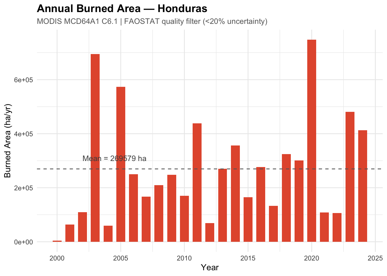
Example: 25 Years of Annual Burned Areas in Honduras

This block builds a 25-year burned-area time series for Honduras, exports it as a data frame, and produces a summary table and bar chart.

# Helper: annual burned area (ha) for one year 
get_annual_ba <- function(year) {
  yr <- as.integer(year)
  annual <- mcd64$
    filter(ee$Filter$calendarRange(yr, yr, "year"))$
    filterBounds(aoi_country_ee$geometry())$
    map(faostat_filter)$
    select("BurnDate")$
    max()$
    gt(0L)$
    selfMask()

  ha <- annual$
    multiply(ee$Image$pixelArea()$divide(10000))$
    reduceRegion(
      reducer   = ee$Reducer$sum(),
      geometry  = aoi_country_ee$geometry(),
      scale     = 500L,
      maxPixels = 1e9
    )$getInfo()

  data.frame(year = yr,
             burned_area_ha = round(ha[["BurnDate"]] %||% 0, 1))
}

# Query all 25 years (~3 min runtime)
years_irl <- 2000:2024
ba_df <- do.call(rbind, lapply(years_irl, get_annual_ba))

# Summary table
knitr::kable(
  ba_df,
  col.names = c("Year", "Burned Area (ha)"),
  caption   = "Annual burned area (MODIS MCD64A1, FAOSTAT filter)",
  align     = c("c", "r")
)

Annual burned area (MODIS MCD64A1, FAOSTAT filter)

Year	Burned Area (ha)
2000	4346
2001	63729
2002	109219
2003	694543
2004	59302
2005	573784
2006	249808
2007	166565
2008	209931
2009	248157
2010	170511
2011	438118
2012	69102
2013	269753
2014	356844
2015	164912
2016	276320
2017	133143
2018	324527
2019	301375
2020	747694
2021	108398
2022	105920
2023	480928
2024	412537

# Bar chart
library(ggplot2)
ggplot(ba_df, aes(x = year, y = burned_area_ha)) +
  geom_col(fill = "#e45a3a", width = 0.7) +
  geom_hline(yintercept = mean(ba_df$burned_area_ha),linetype   = "dashed", colour = "grey40") +
  annotate("text",x = 2002, y = mean(ba_df$burned_area_ha) * 1.15,
                 label = paste0("Mean = ",round(mean(ba_df$burned_area_ha), 0), " ha"),
                 hjust = 0, size = 3.5, colour = "grey30") +
  labs(
    title    = "Annual Burned Area — Honduras",
    subtitle = "MODIS MCD64A1 C6.1 | FAOSTAT quality filter (<20% uncertainty)",
    x = "Year", y = "Burned Area (ha/yr)"
  ) +
  theme_minimal() +
  theme(
    plot.title    = element_text(face = "bold", size = 14),
    plot.subtitle = element_text(size = 10, colour = "gray40")
  )

1.3.2.2 Trend Analysis

# Country-level trend from the ba_df computed above
trend_model <- lm(burned_area_ha ~ year, data = ba_df)
slope  <- coef(trend_model)[["year"]]
pval   <- summary(trend_model)$coefficients["year", "Pr(>|t|)"]

cat("Honduras 2000–2025 — Linear trend in burned area\n")
## Honduras 2000–2025 — Linear trend in burned area
cat("  Slope:", round(slope, 1), "ha/year\n")
##   Slope: 6370 ha/year
cat("  p-value:", signif(pval, 3), "\n")
##   p-value: 0.253
cat("  Interpretation:",
    if (pval < 0.05) "statistically significant" else "not significant",
    "at alpha = 0.05\n")
##   Interpretation: not significant at alpha = 0.05

# Visualise
ggplot(ba_df, aes(x = year, y = burned_area_ha)) +
  geom_col(fill = "#e45a3a", alpha = 0.6, width = 0.7) +
  geom_smooth(method = "lm", se = TRUE,
              colour = "grey30", linewidth = 0.6) +
  labs(
    title    = "Burned Area Trend — Honduras",
    subtitle = paste0("2000–2024 | slope = ",
      round(slope, 1), " ha yr\u207B\u00B9, p = ",
      signif(pval, 2)),
    x = "Year", y = "Burned Area (ha)"
  ) +
  theme_minimal() +
  theme(plot.title = element_text(face = "bold", size = 14))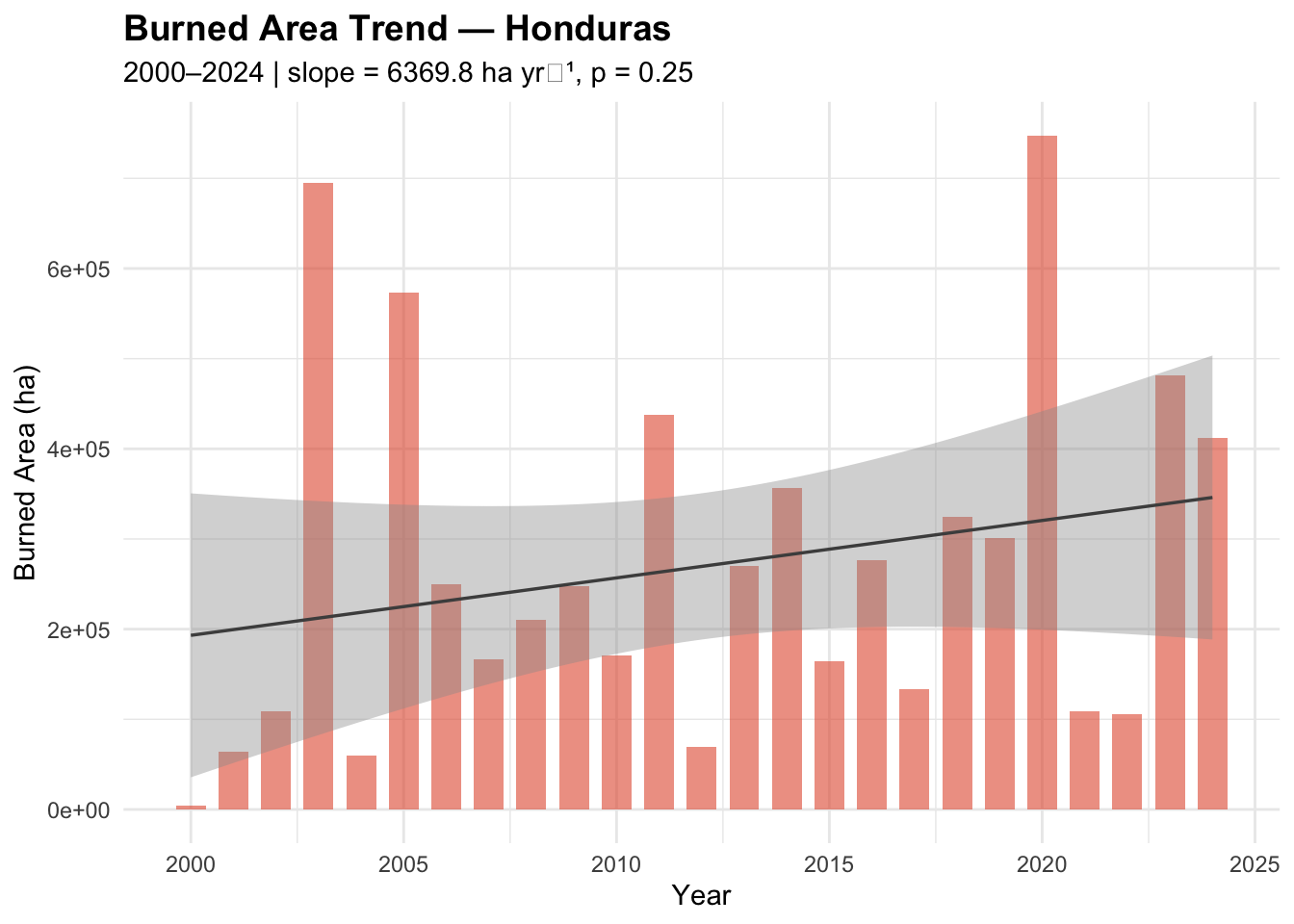

---

1.4 Spatial Aggregation

1.4.1 Country-Level Summaries

1.4.1.1 Using FAO GAUL Boundaries

# Zonal sum: burned area (ha) in 2020
burnedArea_ha <- annual_burned_2020$
  multiply(ee$Image$pixelArea()$divide(10000))$
  reduceRegion(
    reducer   = ee$Reducer$sum(),
    geometry  = aoi_country_ee$geometry(),
    scale     = 500L,
    maxPixels = 1e9
  )$getInfo()

cat("Honduras 2020 — total burned area:",
    round(burnedArea_ha[["burned"]], 1), "ha\n")
## Honduras 2020 — total burned area: 747694 ha

1.4.1.2 Batch Processing for All Countries (Paused)

# Function to calculate burned area for a single country
calculateCountryBA <- function(country_name, year) {
  # Filter country
  country <- countries$filter(ee$Filter$eq("ADM0_NAME", country_name))
  
  # Get annual burned area
  annual_burn <- getAnnualBurn(year)
  
  # Convert to area (hectares)
  burn_area_ha <- annual_burn$
    multiply(ee$Image$pixelArea()$divide(10000))
  
  # Reduce by region
  stats <- burn_area_ha$reduceRegions(
    collection = country,
    reducer = ee$Reducer$sum(),
    scale = 500
  )
  
  # Add metadata
  return(stats$map(function(f) {
    return(f$
      set("year", year)$
      set("country", country_name)
  }))
}

# Process multiple countries and years
country_list <- c("Portugal", "Spain", "France", "Greece")
year_list <- c(2020, 2021, 2022, 2023)

# Create tasks to run in parallel in GEE (250GB per task limit)
for (country in country_list) {
  for (year in year_list) {
    result <- calculateCountryBA(country, year)
    
    # Export task
    task <- ee$batch$Export$table$toDrive(
      collection = result,
      description = paste0(country, "_", year, "_BA"),
      folder = "IPCC_Fire_Emissions",
      fileFormat = "CSV"
    )
    
    task$start()
    print(paste("Started task:", country, year))
  }
}

1.4.2 Sub-National Aggregation

Exercise: Sub-National Aggregation

Aggregate burned area to Honduras’s administrative divisions (departments) using the FAO GAUL level-1 boundaries loaded during GEE setup, then produce a chloropleth map.

# Use the peak fire year for a meaningful map
burn_2020 <- mcd64$
  filter(ee$Filter$calendarRange(2020L, 2020L, "year"))$
  filterBounds(aoi_country_ee$geometry())$
  map(faostat_filter)$
  select("BurnDate")$
  max()$
  gt(0L)$
  selfMask()

# Zonal sum: burned area (ha) per county
county_ba <- burn_2020$
  multiply(ee$Image$pixelArea()$divide(10000))$
  reduceRegions(
    collection = aoi_states_ee,
    reducer    = ee$Reducer$sum(),
    scale      = 500L
  )

# Pull results into R
county_list <- county_ba$getInfo()
county_df <- do.call(rbind, lapply(
  county_list$features, function(f) {data.frame(
      county         = f$properties$ADM1_NAME,
      burned_area_ha = round(f$properties$sum %||% 0, 1))})) |> 
    dplyr::arrange(dplyr::desc(burned_area_ha))

# Summary table
knitr::kable(
  county_df[county_df$burned_area_ha > 0, ],
  col.names = c("County", "Burned Area (ha)"),
  caption   = "Honduras 2020: Burned area by county (non-zero only)",
  row.names = FALSE
)

Honduras 2020: Burned area by county (non-zero only)

County	Burned Area (ha)
Gracias A Dios	256629.1
Olancho	248487.4
Francisco Morazan	91615.2
Paraiso	49749.7
Yoro	29501.3
Comayagua	18784.2
Colon	14393.4
Cortes	13764.0
Choluteca	7868.3
Santa Barbara	5200.9
Copan	3385.3
Intibuca	3225.5
La Paz	1609.2
Valle	1540.8
Atlantida	1034.7
Lempira	842.1
Ocotepeque	48.1

# Choropleth map
county_sf <- dplyr::left_join(
  aoi_states_sf,
  county_df,
  by = c("ADM1_NAME" = "county")
)


ggplot(county_sf) +
  geom_sf(aes(fill = burned_area_ha), colour = "white", linewidth = 0.3) +
  scale_fill_viridis_c(
    name     = "Burned\nArea (ha)",
    option   = "inferno",
    na.value = "grey90") +
  labs(
    title    = "Burned Area by County — Honduras 2020",
    subtitle = "MODIS MCD64A1 C6.1 | FAOSTAT quality filter",
    caption  = "Source: MODIS MCD64A1; Boundaries: FAO GAUL level-1") +
  theme_void() +
  theme(
    plot.title    = element_text(face = "bold", size = 14),
    plot.subtitle = element_text(size = 10, colour = "gray40"))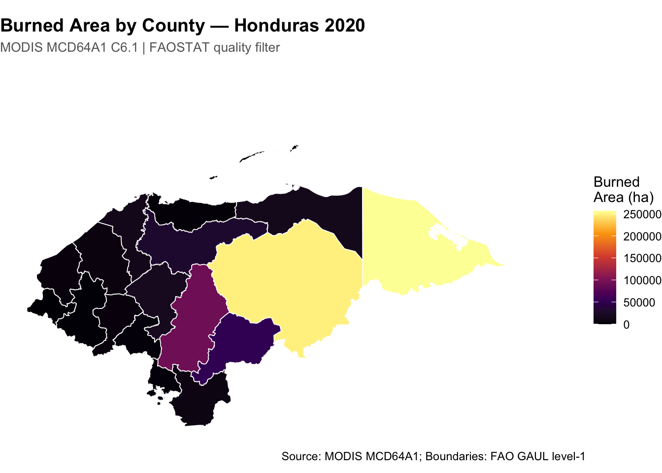

1.4.3 Area Calculation Corrections

Latitude correction for pixel area:

# Standard approach: Use ee.Image.pixelArea()
# This automatically accounts for latitude

# Manual calculation (for understanding):
calculatePixelArea <- function(image) {
  # Get latitude for each pixel
  lat <- ee$Image$pixelLonLat()$select("latitude")
  
  # Convert to radians
  lat_rad <- lat$multiply(pi / 180)
  
  # Pixel height (constant in sinusoidal projection)
  pixel_height_m <- ee$Image$constant(463.3127)  # meters at equator for 500m product

  # Pixel width varies with latitude
  pixel_width_m <- pixel_height_m$multiply(lat_rad$cos())

  # Area in m²
  pixel_area_m2 <- pixel_height_m$multiply(pixel_width_m)
  
  return(pixel_area_m2)
}

# Compare with built-in function
pixel_area_builtin <- ee$Image$pixelArea()
pixel_area_manual <- calculatePixelArea()

---

1.5 Multi-Source Validation

1.5.1 GLAD Comparison

# Forest mask from MCD12Q1 (IGBP classification)
# Classes 1-5 = forest types (Evergreen Needleleaf, Evergreen Broadleaf,
# Deciduous Needleleaf, Deciduous Broadleaf, Mixed Forest)
lc <- ee$ImageCollection("MODIS/061/MCD12Q1")$
  filterDate("2020-01-01", "2020-12-31")$first()$
  select("LC_Type1")
forest_mask <- lc$lte(5L)$And(lc$gte(1L))$clip(aoi_country_ee$geometry())

# GLAD canopy height in GEE
glad_height <- ee$Image("UMD/hansen/global_forest_change_2023_v1_11")$
  select("treecover2000")

# Forest threshold: > 25% canopy cover. 
# Reproject to MODIS grid with upsampling 
glad_forest <- glad_height$gt(25L)
glad_forest_500m <- glad_forest$reproject(crs = modis_proj, scale = 500L)

# forest_mask at MODIS native res 
modis_forest_binary <- forest_mask$unmask(0L)$
  reproject(crs = modis_proj, scale = 500L)
glad_forest_binary  <- glad_forest_500m$unmask(0L)

agreement  <- modis_forest_binary$And(glad_forest_binary)
modis_only <- modis_forest_binary$And(glad_forest_binary$Not())
glad_only  <- glad_forest_binary$And(modis_forest_binary$Not())

val_stats <- ee$Image$cat(
  agreement$rename("agree"),
  modis_only$rename("modis_only"),
  glad_only$rename("glad_only")
)$reduceRegion(
  reducer   = ee$Reducer$sum(),
  geometry  = aoi_country_ee$geometry(),
  scale     = 500L,
  maxPixels = 1e9,
    bestEffort = TRUE)$getInfo()

total <- as.integer(val_stats$agree %||% 0) +
  as.integer(val_stats$modis_only %||% 0) +
  as.integer(val_stats$glad_only %||% 0)

cat("Honduras — Forest Classification Agreement\n")
## Honduras — Forest Classification Agreement
cat("  Both agree (forest):  ", val_stats$agree, "pixels\n")
##   Both agree (forest):   110610 pixels
cat("  MODIS-only forest:    ", val_stats$modis_only, "pixels\n")
##   MODIS-only forest:     2681 pixels
cat("  Hansen-only forest:   ", val_stats$glad_only, "pixels\n")
##   Hansen-only forest:    236694 pixels
if (total > 0) {cat("  Agreement rate: ",round(as.integer(
    val_stats$agree %||% 0) / total * 100, 1), "%\n")}
##   Agreement rate:  31.6 %

# Visualize agreement
tmap::tm_shape(aoi_country_sf) + tmap::tm_borders(col = "white", lwd = 1.5) +
  tmap::tm_tiles(ee_tile_url(agreement$selfMask()$clip(aoi_country_ee$geometry()),
      list(palette = "green", min = 1L, max = 1L)), group = "Both Agree: Forest") +
  tmap::tm_tiles(ee_tile_url(modis_only$selfMask()$clip(aoi_country_ee$geometry()),
      list(palette = "blue", min = 1L, max = 1L)), group = "MODIS-only Forest") +
  tmap::tm_tiles(ee_tile_url(glad_only$selfMask()$clip(aoi_country_ee$geometry()),
      list(palette = "red", min = 1L, max = 1L)), group = "Hansen-only Forest") +
  tmap::tm_add_legend(type = "polygons", fill = c("green", "blue", "red"),
      labels = c("Both Agree: Forest", "MODIS-only Forest", "Hansen-only Forest"),
      title = "Forest Cover Agreement") +
    tmap::tm_scalebar(position = c("RIGHT", "BOTTOM"), text.size = 0.5) +
  tmap::tm_basemap("Esri.WorldImagery")

1.5.2 ESA WorldCover Validation

# ESA WorldCover 2020 (10m) in GEE
# Do NOT clip() 10m data — materialises >2^31 pixels over Honduras
# Reproject to MODIS 500m grid IMMEDIATELY at load time
# Using shared modis_proj from init chunk

esa_2020 <- ee$Image("ESA/WorldCover/v100/2020")$
  reproject(crs = modis_proj, scale = 500L)

# ESA classes: 10=Tree cover, 20=Shrubland, 30=Grassland,
# 40=Cropland, 50=Built-up, 60=Bare, 70=Snow/Ice,
# 80=Water, 90=Herbaceous wetland, 95=Mangroves, 100=Moss/Lichen

# ESA forest (Tree cover)
esa_forest <- esa_2020$eq(10L)

# ESA savanna proxy (Shrubland + Grassland)
esa_savanna <- esa_2020$eq(20L)$Or(esa_2020$eq(30L))

# Compare ESA forest with MODIS forest
# Both images are already at 500m (esa_2020 reprojected above,
# forest_mask from MCD12Q1 native 500m) — safe to unmask and combine
esa_forest_binary <- esa_forest$unmask(0L)$
  reproject(crs = modis_proj, scale = 500L)
modis_forest_500m <- forest_mask$unmask(0L)$
  reproject(crs = modis_proj, scale = 500L)

agree_esa  <- modis_forest_500m$And(esa_forest_binary)
modis_esa  <- modis_forest_500m$And(esa_forest_binary$Not())
esa_only   <- esa_forest_binary$And(modis_forest_500m$Not())

esa_stats <- ee$Image$cat(
  agree_esa$rename("agree"),
  modis_esa$rename("modis_only"),
  esa_only$rename("esa_only")
)$reduceRegion(
  reducer   = ee$Reducer$sum(),
  geometry  = aoi_country_ee$geometry(),
  scale     = 500L,
  maxPixels = 1e9,
    bestEffort = TRUE)$getInfo()

cat("Honduras — MODIS vs ESA WorldCover Forest Agreement\n")
## Honduras — MODIS vs ESA WorldCover Forest Agreement
cat("  Overlapping forest: ", esa_stats$agree, "pixels\n")
##   Overlapping forest:  104910 pixels
cat("  MODIS-only forest:   ", esa_stats$modis_only, "pixels\n")
##   MODIS-only forest:    8381 pixels
cat("  ESA-only forest:     ", esa_stats$esa_only, "pixels\n")
##   ESA-only forest:      204323 pixels

---

1.6 Uncertainty Reporting

1.6.1 Quantifying Total Uncertainty

Following IPCC guidelines, uncertainty in burned area activity data combines:

\[ U_{total}^2 = U_{detection}^2 + U_{classification}^2 + U_{area}^2 \]

Where:

• \(U_{detection}\) = Omission/commission errors in fire detection
• \(U_{classification}\) = Land cover misclassification affecting fire-prone area
• \(U_{area}\) = Geometric/projection errors in area calculation

Typical values for MODIS MCD64A1:

• Detection uncertainty: ±25-35% (varies by biome)
• Classification uncertainty: ±10-15% (from MCD12Q1 validation)
• Area uncertainty: ±2-5% (projection and edge effects)

Combined uncertainty: Approximately ±30% for global Tier 1 applications

1.6.2 Sensitivity Analysis

# Use full MCD64A1 collection — not a pre-filtered subset
mcd64_sens <- ee$ImageCollection("MODIS/061/MCD64A1")$
  filterDate("2020-01-01", "2020-12-31")$
  filterBounds(aoi_country_ee$geometry())
geom <- aoi_country_ee$geometry()

# Test multiple uncertainty thresholds
thresholds <- c(10L, 15L, 20L, 25L, 30L)

sensitivity_results <- do.call(rbind, lapply(thresholds, function(thresh) {
  tryCatch({
    filtered <- mcd64_sens$map(function(img) {
      mask <- img$select("Uncertainty")$lt(thresh)$
        And(img$select("BurnDate")$gt(0L))
      img$updateMask(mask)
    })

    result <- filtered$
      select("BurnDate")$max()$gt(0L)$selfMask()$
      multiply(ee$Image$pixelArea()$divide(10000))$
      reduceRegion(
        reducer    = ee$Reducer$sum(),
        geometry   = geom,
        scale      = 500L,
        maxPixels  = 1e9,
        bestEffort = TRUE
      )$getInfo()

    val <- result[["BurnDate"]]
    data.frame(
      threshold      = thresh,
      burned_area_ha = if (is.null(val)) NA_real_ else as.numeric(val)
    )
  }, error = function(e) {
    message("Threshold ", thresh, " failed: ", e$message)
    data.frame(threshold = thresh, burned_area_ha = NA_real_)
  })
}))

ggplot(sensitivity_results, aes(x = threshold, y = burned_area_ha)) +
  geom_line(linewidth = 1, color = "darkred") +
  geom_point(size = 3, color = "darkred") +
  geom_vline(xintercept = 20, linetype = "dashed", color = "blue") +
  annotate("text", x = 20,
           y = max(sensitivity_results$burned_area_ha, na.rm = TRUE) * 0.9,
           label = "FAOSTAT threshold", hjust = -0.1) +
  scale_y_continuous(labels = scales::comma) +
  labs(
    title = "Sensitivity of Burned Area to Uncertainty Threshold",
    subtitle = "Honduras 2020 — MCD64A1",
    x = "Uncertainty Threshold (%)",
    y = "Burned Area (hectares)"
  ) +
  theme_minimal()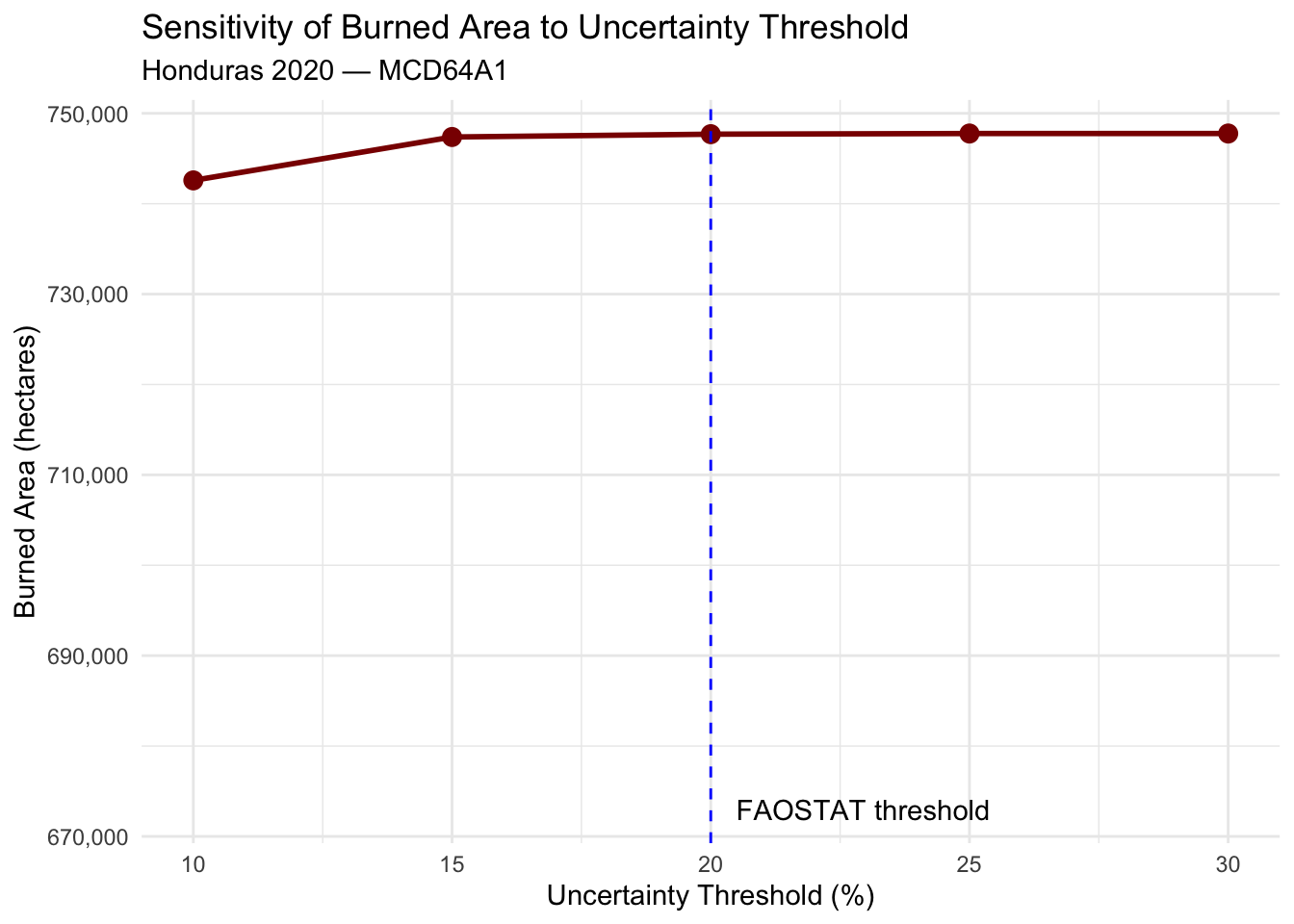

1.6.3 Documenting Uncertainty for NGHGI

Required documentation:

1. Data source and version: MODIS MCD64A1 Collection 6.1
2. Quality criteria applied: Uncertainty < 20%
3. Spatial coverage: Percentage of country with valid observations
4. Temporal coverage: Months with cloud-free observations
5. Estimated uncertainty: ±30% (or country-specific if available)
6. Validation results: Comparison with independent data sources

Example uncertainty table for NGHGI report:

uncertainty_table <- data.frame(
  Source = c(
    "Satellite detection",
    "Land cover classification",
    "Area calculation",
    "Total (quadrature)"),
  Uncertainty = c("\u00b130%", "\u00b115%", "\u00b15%", "\u00b134%"),
  Method = c(
    "MCD64A1 validation (Giglio et al. 2018)",
    "MCD12Q1 accuracy assessment",
    "Projection error analysis",
    "IPCC Equation 3.1"
  )
)

knitr::kable(
  uncertainty_table,
  caption = "Uncertainty of Burned Area Activity Data",
  align = c("l", "c", "l")
)

Uncertainty of Burned Area Activity Data

Source	Uncertainty	Method
Satellite detection	±30%	MCD64A1 validation (Giglio et al. 2018)
Land cover classification	±15%	MCD12Q1 accuracy assessment
Area calculation	±5%	Projection error analysis
Total (quadrature)	±34%	IPCC Equation 3.1

---

1.7 Reproducible Workflow

1.7.1 Consolidated Script

# IPCC Tier 1 Burned Area Processing Script
# ============================================================

# 1. Parameters
year_start <- 2000L
year_end   <- 2024L

# 2. Temporal Aggregation
getAnnualBurn <- function(yr) {
  annual <- burned_area$
    filter(ee$Filter$calendarRange(yr, yr, "year"))$map(filterQuality)$
    select("BurnDate")$max()$gt(0L)$selfMask()
  annual$set("year", yr)$set("system:time_start", ee$Date$fromYMD(yr, 1L, 1L)$millis())
  }

years <- seq(year_start, year_end, 1L)
annual_collection <- ee$ImageCollection(lapply(years, getAnnualBurn))

# 3. Spatial Aggregation
calculateBA <- function(image) {
  yr <- image$get("year")
  area_ha <- image$
    multiply(ee$Image$pixelArea()$divide(10000))$
    reduceRegion(
      reducer   = ee$Reducer$sum(),
      geometry  = aoi_country_ee$geometry(),
      scale     = 500L,
      maxPixels = 1e9)
  ee$Feature(NULL, list(
    year = yr,
    country = "Honduras",
    burned_area_ha = area_ha$get("BurnDate")))
  }

results <- annual_collection$map(calculateBA)

# 4. Export Results
task <- ee$batch$Export$table$toDrive(
  collection  = results,
  description = paste0("Honduras_BA_", year_start, "_", year_end),
  folder      = "IPCC_Fire_Emissions",
  fileFormat  = "CSV"
)

# Export task disabled
#task$start()
#cat("Export started:", task$id, "\n")

# Or pull directly into R
results_df <- ee_to_sf(results) |> sf::st_drop_geometry()
print(results_df)

# 5. Visualization
ggplot(results_df, aes(x = year, y = burned_area_ha)) +
  geom_line(color = "darkred", linewidth = 1) +
  geom_point(color = "darkred", size = 3) +
  labs(
    title    = "Annual Burned Area — Honduras", 
    subtitle = paste("MODIS MCD64A1 Collection 6.1 |", year_start, "–", year_end),
    x = "Year", y = "Burned Area (hectares)") +
  theme_minimal() +
  theme(plot.title=element_text(face="bold",size=14),plot.subtitle = element_text(size=10,color="gray40"))

1.7.2 Output Format

For NGHGI Reporting:

# Create IPCC-compatible output table
nghgi_output <- results_df %>%
  mutate(
    Category = "4.C Forest Land",
    Subcategory = "Fires on Forest Land",
    Activity_Data_Unit = "ha",
    Data_Source = "MODIS MCD64A1 Collection 6.1",
    Quality_Tier = "Tier 1",
    Uncertainty_Percent = 30
    ) %>%
  rename(
    Year = year,
    Country = country,
    Burned_Area_ha = burned_area_ha
    )

# Export
write.csv(
  nghgi_output,
  file = paste0(country_name, "_BurnedArea_NGHGI_", Sys.Date(), ".csv"),
  row.names = FALSE
)

1.7.3 QC Checklist

Pre-processing:

• GEE authentication successful
• AOI geometry valid (no self-intersections)
• Date range covers complete years
• Image collection not empty

Processing:

• Quality filter applied (uncertainty < 20%)
• Temporal aggregation complete (12 months per year)
• Spatial aggregation uses correct boundaries (EUROSTAT, 2026)
• Area calculation accounts for projection

Post-processing:

• No missing years in time series
• Burned area values reasonable (order of magnitude check)
• Comparison with previous estimates (if available)
• Validation with independent data
• Uncertainty quantified and documented

Reporting:

• Data source and version documented
• Methods transparent and reproducible
• Code archived in version control
• Results exported in standard format
• Metadata complete (CRS, resolution, quality flags)

---

EUROSTAT. (2026). Geographic information system of the european commission.

Giglio, L., Boschetti, L., Roy, D. P., Humber, M. L., & Justice, C. O. (2018). The collection 6 MODIS burned area mapping algorithm and product. Remote Sensing of Environment, 217, 72–85.

Rossi, S., Tubiello, F. N., Prosperi, P., Salvatore, M., Jacobs, H., Biancalani, R., House, J. I., & Boschetti, L. (2016). FAOSTAT estimates of greenhouse gas emissions from biomass and peat fires. Climatic Change, 135(3), 699–711.