
download.file(
  url      = "https://data.hydrosheds.org/file/HydroBASINS/customized_with_lakes/hybas_lake_na_lev06_v1c.zip",
  destfile = "./assets/SHP/watersheds_na_l6.zip",
  mode     = "wb"
  )

unzip(
  zipfile = "./assets/SHP/watersheds_na_l6.zip",
  exdir   = "./assets/SHP/"
  )

xy         = "49.95,-119.43"
watersheds = sf::st_read("./assets/SHP/watersheds_na_l6/hybas_lake_na_lev06_v1c.shp")
aoi_xy     = sf::st_read("./assets/SHP/aoi_xy.shp")
aoi        = watersheds |> sf::st_intersection(aoi_xy)
sf::st_write(aoi, "./assets/SHP/aoi_watershed.shp")

tmap::tmap_mode("view")
tmap::tm_shape(aoi) + tmap::tm_borders(col="purple", lwd=2) +
  tmap::tm_scalebar(position=c("RIGHT", "BOTTOM"), text.size = .5) +
tmap::tm_title("AOI Waterhsed", size=.8) CFFDRS 2.0: Canadian Forest Fire Danger Rating System Updated
Reproducible pipeline for forest fuel typing and fire risk metrics in British Columbia’s Okanagan Watershed in accordance with updated CFFDRS V2.0
Abstract
This report documents development of wildfire risk mapping and behavior prediction metrics in accordance with the Canadian Forest Fire Danger Rating System (V2.0). Leveraging the new cffdrs package and the release of the updated Fire Danger Rating System framework, the following demonstrates a reproducible and technically aligned workflow to data acquisition, spatial covariate processing, including satellite-derived elevation, gridded climate data, and vegetation inventories, to produce fire behavior outputs. The methodology is designed to support the needs of fire managers, researchers, andwildfire operational teams by providing robust estimates of current day fire environment. This markdown was originally commissioned for preparation of submission to the Innovative Solutions Canada grant funding and was since updated with releases of new input data.
Keywords
Wildfire Risk, Fuel Typing, Canadian Forest Fire Danger Rating System (V2.0)
1. Introduction
The Canadian Forest Fire Danger Rating System (CFFDRS) has served as the scientific foundation for wildland fire management in Canada. The next generation of the CFFDRS (V2.0) includes several enhancements designed to incorporate new data sources and address the increasing complexity of contemporary fire management (Boucher et al., n.d.). This report provides a reproducible pipeline using the cffdrs R package to derive key fire behavior metrics. Our workflow develops raster layers of fuel moisture codes and wildfire weather indices. These inputs are used to inform the stand-adjusted fine-fuel model (Wotton and Beverly 2007) and classify vegetation into fuel classes based on the BC forest fuel typing framework (D. D. Perrakis, Eade, and Hicks 2018; D. D. Perrakis et al. 2023). The resulting fuel type rasters are compiled to predict fire behavior, from which we derive Head Fire Index (HFI) and Fire Intensity (FI) maps for the Okanagan Watershed Basin for the 2021 fire season. The full workflow is illustrated in the flowchart below.

Clone repository
This guide enables reproducible analysis by cloning the supporting repository using the following bash commands in your terminal:
git clone https://github.com/seamusrobertmurphy/wildfire-fuel-mapping-CFFDRS-2.0.git2. Method
Import AOI Data
Two input options for selecting AOI were explored below: 1) uploading AOI boundary file and 2) choosing point location as centre of 10km LxW bounding box. We downloaded the Okanagan Watershed boundary (FWA ID:212) and transformed into spatVector for implementing workflow using terra functions.
Import DEM Data
Topography is a primary driver of fire behavior, influencing fire spread, intensity, and fuel moisture. This section details a reproducible workflow for acquiring Digital Elevation Model (DEM) data and its derivatives. The following chunk begins by acquiring a DEM raster for the AOI using the elevatr package (Hollister et al. 2023). From this dataset, slope and aspect rasters were derived. All three layers were then processed using the terra package to ensure a consistent spatial alignment and extent. Make sure to toggle layers on and off to inspect visually.
elev  = elevatr::get_elev_raster(aoi, z=11) # res==zoom -> https://github.com/tilezen/joerd/blob/master/docs/data-sources.md#what-is-the-ground-resolution
raster::writeRaster(elev, "./assets/TIF/elevation.tif", overwrite=T)

slope = raster::terrain(elev,
  opt       = "slope",
  neighbors = 8,
  overwrite = T,
  filename  = "./assets/TIF/slope.tif"
  )

aspect = raster::terrain(elev,
  opt       = "aspect",
  neighbors = 8,
  overwrite = T,
  filename  = "./assets/TIF/aspect.tif"
  )

# Tidy elevation rasters
elev  = terra::rast("./assets/TIF/elevation.tif") |> terra::project("EPSG:3857")
slope = terra::rast("./assets/TIF/slope.tif") |> terra::project("EPSG:3857")
aspect= terra::rast("./assets/TIF/aspect.tif") |> terra::project("EPSG:3857")
slope = terra::resample(slope, elev, method="bilinear")
aspect= terra::resample(aspect, elev, method="bilinear")
slope = terra::mask(slope, terra::vect(sf::st_transform(aoi, "EPSG:3857")))
aspect= terra::mask(aspect, terra::vect(sf::st_transform(aoi, "EPSG:3857")))
elev  = terra::mask(elev, terra::vect(sf::st_transform(aoi, "EPSG:3857")))
raster::writeRaster(elev, "./assets/TIF/elevation.tif", overwrite=T)
raster::writeRaster(slope, "./assets/TIF/slope.tif", overwrite=T)
raster::writeRaster(aspect, "./assets/TIF/aspect.tif", overwrite=T)


tmap::tm_shape(elev)+ tm_raster(
    style= "cont", title="Elevation ASL", palette="viridis")+
  tmap::tm_shape(slope)+ tm_raster(
    style= "cont", title="Slope", palette="Oranges") +
  tmap::tm_shape(aoi)+ tm_borders(col="purple", lwd = 2) +
  tmap::tm_compass(type = "8star", position = c("left", "top")) +
  tmap::tm_scale_bar(c(0, 10, 20, 40), position = c("RIGHT", "BOTTOM"), text.size = .5) +
  tmap::tm_title("Elevation Rasters", size=0.8) +
tmap::tm_basemap("Esri.WorldImagery") 
Import Climate Data
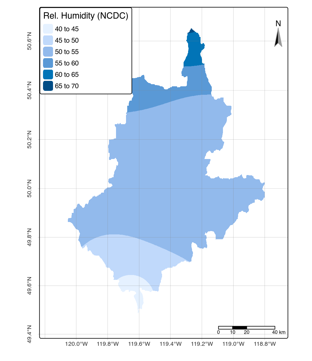
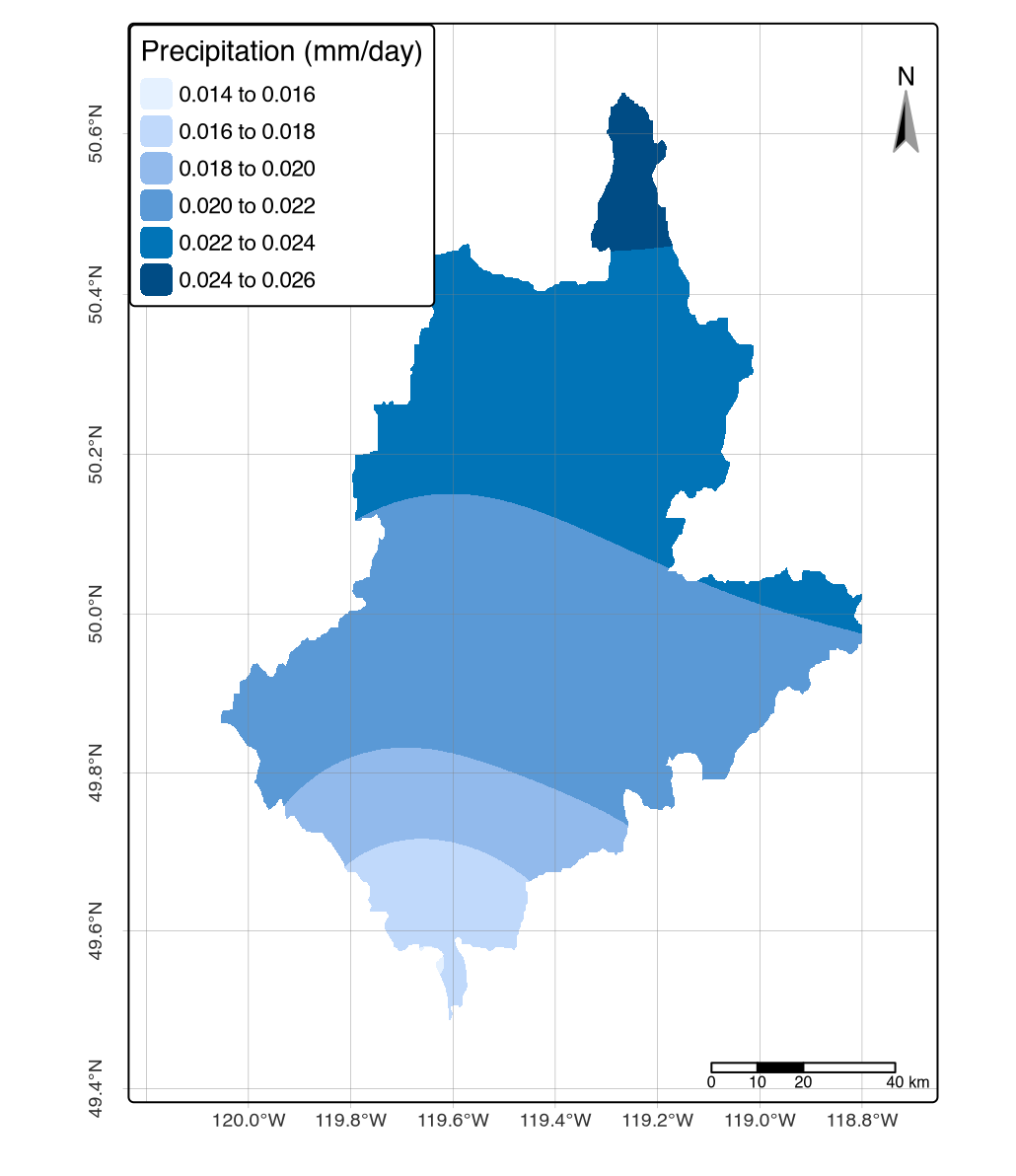
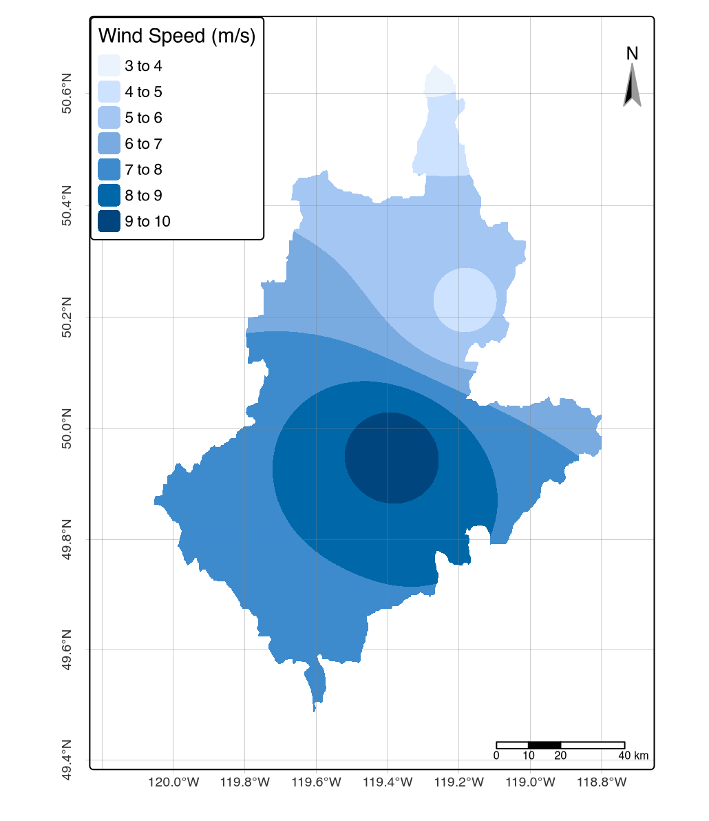
Climate data, a fundamental input for wildfire weather calculations, is sourced from Environment and Climate Change Canada using the weathercan package. This approach replaces the manual data sourcing from platforms with reproducible, verifiable solution. The workflow begins by searching for all weather stations within a specified radius of the AOI. Hourly data for these stations is downloaded for the defined date range and then aggregated to a single mean value for each station for the target period. The cleaned, point-based spatial data is converted into continuous raster layers for each input variable, which are derived using Inverse Distance Weighting (IDW) method via a gstat model and the terra::interpolate function. The resulting outputs of mean daily temperature, precipitation, relative humidity, and wind speed are then masked to the AOI and saved for use in the next stages of the analysis.
# Search weather stations
stations_100km = weathercan::stations_search(
  coords  = c(49.95,-119.43),
  interval= "day",
  dist    = 100)

# Parse by station
stations_ids_unique <- stations_100km |>
  dplyr::pull(station_id) |> unique()

# Download data for all selected stations
climate_tbl <- weathercan::weather_dl(
  station_ids = stations_ids_unique,
  start = "2021-06-01",
  end = "2021-10-01",
  interval = "hour") # relative humidity in hourly only

# Aggregate by station
aggregated_data <- climate_tbl |>
  dplyr::group_by(station_id, lat, lon) |>
  dplyr::summarise(
    mean_temp = mean(temp, na.rm = TRUE),
    mean_prec = mean(prec_amt, na.rm = TRUE),
    mean_rh   = mean(rel_hum, na.rm = TRUE),
    mean_ws   = mean(wind_spd, na.rm = TRUE)
  ) |>
  dplyr::ungroup()

# Convert to spatial and filter missing stations
climate_sf <- aggregated_data |>
  dplyr::filter(
    !is.nan(mean_temp),
    !is.nan(mean_prec),
    !is.nan(mean_rh),
    !is.nan(mean_ws)
  ) |>
  sf::st_as_sf(
    coords = c("lon", "lat"),
    crs = 4326
  ) |>
  sf::st_transform("EPSG:3857")

# Derive raster template to interpolate on top of
raster_template <- terra::rast("./assets/TIF/elevation.tif")

# Derive function to handle `sf` weather station data
interpolate_stations <- function(model, x, crs, ...) {
    v <- st_as_sf(x, coords = c("x", "y"), crs = crs)
    p <- predict(model, v, ...)
    as.data.frame(p)[, 1:2]
  }

# Create Inverse Distance Weighting models using gstat.pkg
temp_idw <- gstat(
  formula = mean_temp ~ 1,
  locations = climate_sf,
  nmax = 8,
  set = list(idp = 2.0)
  )

prec_idw <- gstat(
  formula = mean_prec ~ 1,
  locations = climate_sf,
  nmax = 8,
  set = list(idp = 2.0)
  )

rh_idw <- gstat(
  formula = mean_rh ~ 1,
  locations = climate_sf,
  nmax = 8,
  set = list(idp = 2.0)
  )

ws_idw <- gstat(
  formula = mean_ws ~ 1,
  locations = climate_sf,
  nmax = 8,
  set = list(idp = 2.0)
  )


# Spatially interpolate using terra.pkg
temp_rast <- terra::interpolate(
  object = raster_template,
  model = temp_idw,
  fun = interpolate_stations,
  crs = "EPSG:3857",
  debug.level = 0
)

prec_rast <- terra::interpolate(
  object = raster_template,
  model = prec_idw,
  fun = interpolate_stations,
  crs = "EPSG:3857",
  debug.level = 0
)

rh_rast <- terra::interpolate(
  object = raster_template,
  model = rh_idw,
  fun = interpolate_stations,
  crs = "EPSG:3857",
  debug.level = 0
)

ws_rast <- terra::interpolate(
  object = raster_template,
  model = ws_idw,
  fun = interpolate_stations,
  crs = "EPSG:3857",
  debug.level = 0
)

# Tidy, save, and visualize
temp    = terra::mask(temp_rast, terra::vect(sf::st_transform(aoi, "EPSG:3857")))
prec    = terra::mask(prec_rast, terra::vect(sf::st_transform(aoi, "EPSG:3857")))
rh      = terra::mask(rh_rast, terra::vect(sf::st_transform(aoi, "EPSG:3857")))
ws      = terra::mask(ws_rast, terra::vect(sf::st_transform(aoi, "EPSG:3857")))

terra::writeRaster(temp, "./assets/TIF/temp.tif", overwrite=T)
terra::writeRaster(prec, "./assets/TIF/prec.tif", overwrite=T)
terra::writeRaster(rh, "./assets/TIF/rh.tif", overwrite=T)
terra::writeRaster(ws, "./assets/TIF/ws.tif", overwrite=T)

tmap::tmap_mode("plot")
tmap::tm_shape(temp)+ tm_raster(style= "cont",
  title="Mean Daily Temperature (°C 2m AGL)", palette="Oranges")+
  tmap::tm_shape(aoi)+ tm_borders(col="purple", lwd = 2) +
  tmap::tm_compass(color.dark="gray60",text.color="gray60",position=c("RIGHT","top"))+
  tmap::tm_graticules(lines=T,labels.rot=c(0,90),lwd=0.2) +
  tmap::tm_scale_bar(c(0, 10, 20, 40), position = c("RIGHT", "BOTTOM"), text.size = .5)

tmap::tm_shape(prec)+ tm_raster(style= "cont",
  title="Mean Daily Precipitation (mm^3/day)", palette="Oranges") +
  tmap::tm_shape(aoi)+ tm_borders(col="purple", lwd = 2) +
  tmap::tm_compass(color.dark="gray60",text.color="gray60",position=c("RIGHT","top"))+
  tmap::tm_graticules(lines=T,labels.rot=c(0,90),lwd=0.2) +
  tmap::tm_scale_bar(c(0, 10, 20, 40), position = c("RIGHT", "BOTTOM"), text.size = .5)

tmap::tm_shape(rh)+ tm_raster(style= "cont",
  title="Relative Humidity (NCDC 2m AGL)", palette="Oranges") +
  tmap::tm_shape(aoi)+ tm_borders(col="purple", lwd = 2) +
  tmap::tm_compass(color.dark="gray60",text.color="gray60",position=c("RIGHT","top"))+
  tmap::tm_graticules(lines=T,labels.rot=c(0,90),lwd=0.2) +
  tmap::tm_scale_bar(c(0, 10, 20, 40), position = c("RIGHT", "BOTTOM"), text.size = .5)

tmap::tm_shape(ws)+ tm_raster(style= "cont",
  title="Wind Speed (m/s 10m AGL)", palette="Oranges") +
  tmap::tm_shape(aoi)+ tm_borders(col="purple", lwd = 2) +
  tmap::tm_compass(color.dark="gray60",text.color="gray60",position=c("RIGHT","top"))+
  tmap::tm_graticules(lines=T,labels.rot=c(0,90),lwd=0.2) +
tmap::tm_scale_bar(c(0, 10, 20, 40), position = c("RIGHT", "BOTTOM"), text.size = .5) 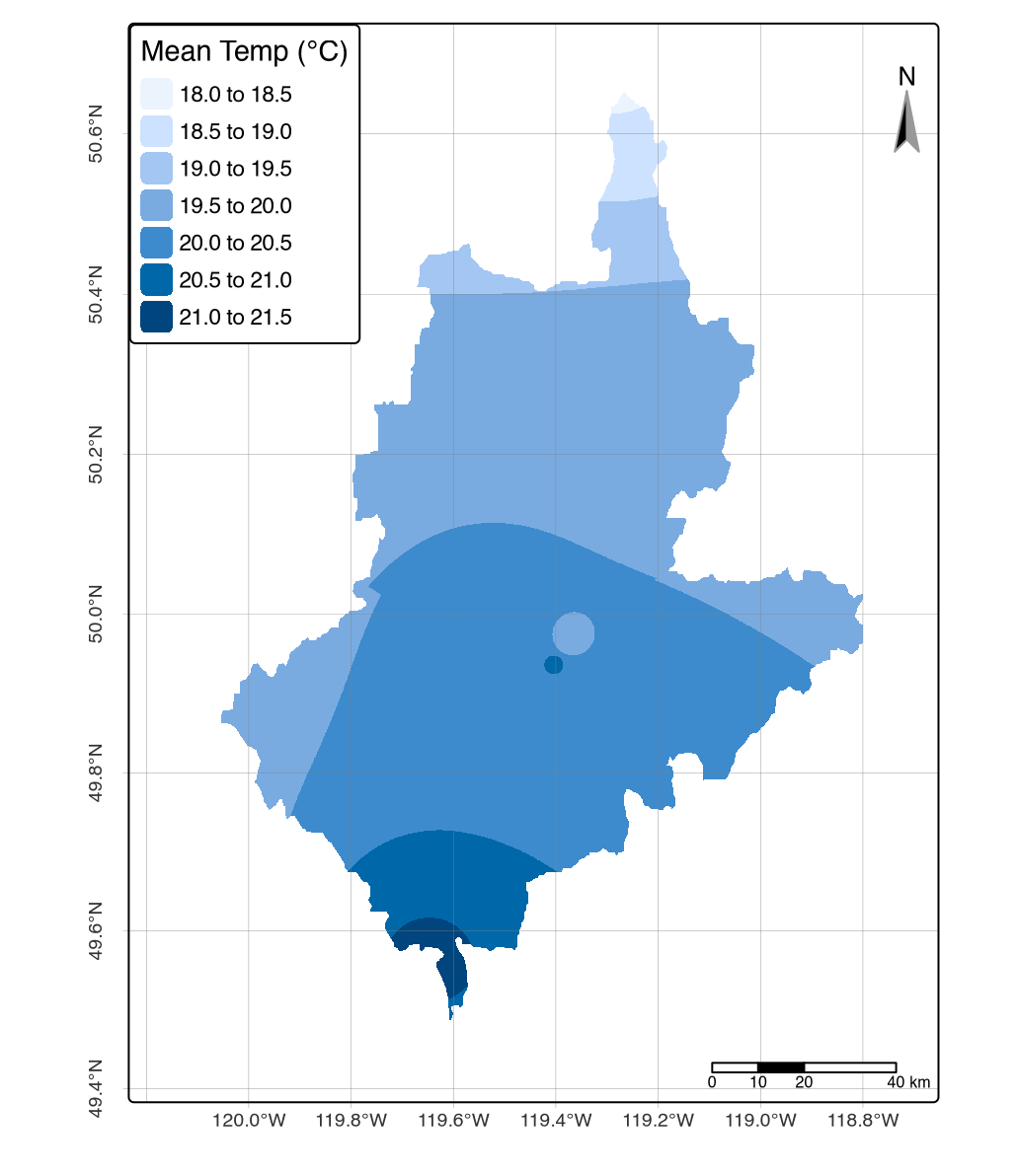 |
 |
 |
 |
3. Results
Derive Fuel Type Maps
The Fire Behavior Prediction (FBP) system relies on a detailed and accurate classification of fuel types. This section demonstrates development of fuel maps from the publicly available BC Vegetation Resource Inventory (VRI) dataset downloaded from BC Data Catalog.
To ensure our inputs are correctly formatted for the cffdrs package, we reviewed the included example datasets, test_fwi and test_fbp, which serve as templates guiding input requirements and structure, as documented in the VRI data dictionary here.
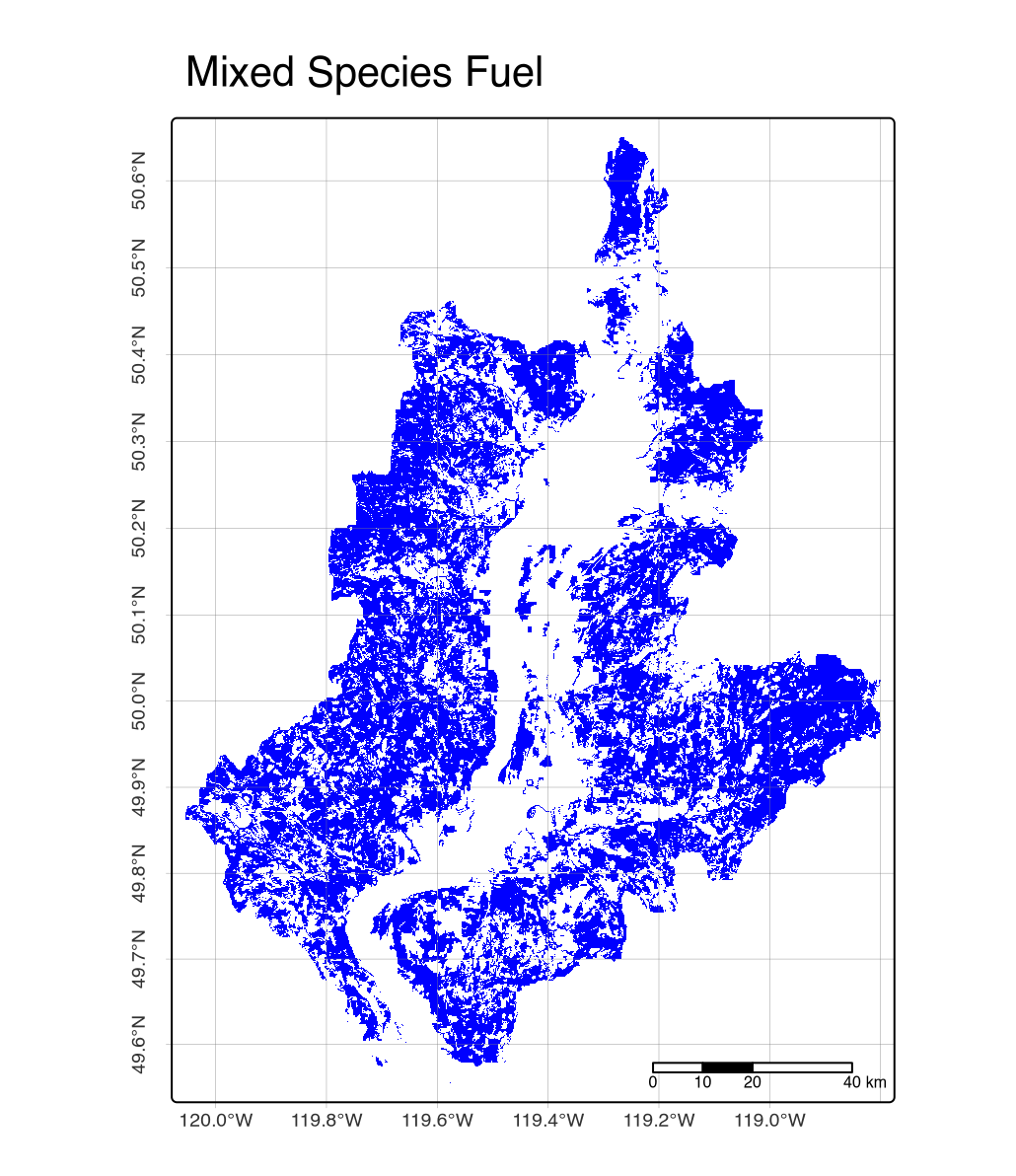
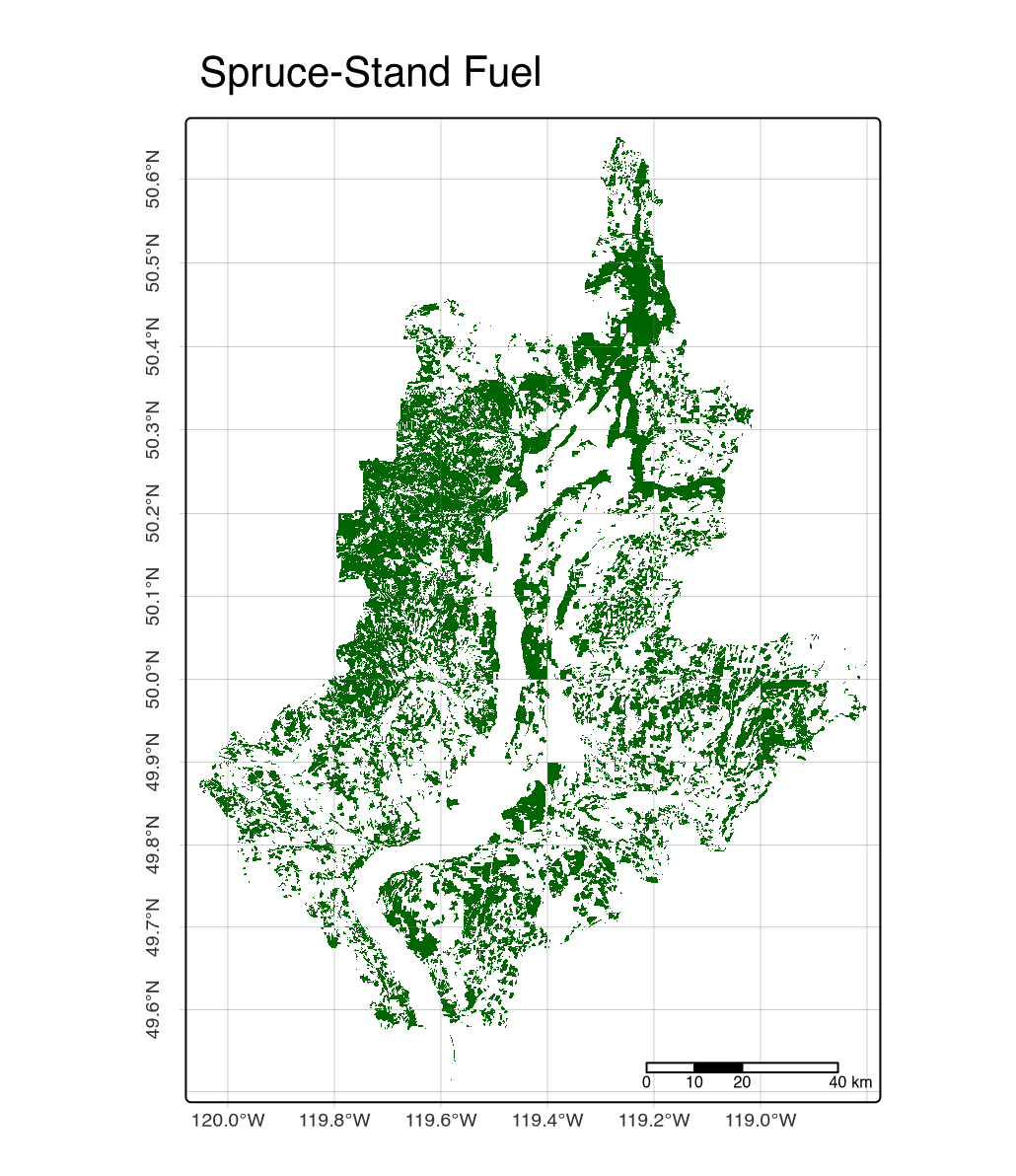
Following the workflow of Wotton and Beverly’s stand-adjusted fine-fuel moisture model (Wotton and Beverly 2007) and more recent methodologies (D. D. Perrakis, Eade, and Hicks 2018), we classified the VRI attributes into distinct fuel categories. This process extracted predictor variables, such as stand type and density, and applied a filtering process to classify fuel categories that are consistent with the FBP system. The resulting classified vector layers serve as the foundational fuel maps for all subsequent fire behavior predictions.
# Download
download.file(destfile = "./assets/VRI/vri_2024.zip", mode = "wb",
  url = "https://pub.data.gov.bc.ca/datasets/02dba161-fdb7-48ae-a4bb-bd6ef017c36d/current/VEG_COMP_POLY_AND_LAYER_2024.gdb.zip")
unzip(zipfile = "./assets/VRI/vri_2024.zip",
  exdir = "./assets/VRI/")

# Tidy & save
vri_2024  = sf::st_read("./assets/VRI/vri_2024.shp") |>
  sf::st_intersects(sf::st_transform(aoi, "EPSG:3005")) |>
  sf::st_transform("EPSG:3857")
sf::st_write(vri_2024, ".assets/VRI/vri_2024_3857.shp")

# Input Requirements
library(cffdrs)
print(as_tibble(test_fwi), n = 10)
print(as_tibble(test_fbp), n = 10)
NA # A tibble: 48 × 9
NA long lat yr mon day temp rh ws prec
NA <int> <int> <int> <int> <int> <dbl> <int> <int> <dbl>
NA 1 -100 40 1985 4 13 17 42 25 0
NA 2 -100 40 1985 4 14 20 21 25 2.4
NA 3 -100 40 1985 4 15 8.5 40 17 0
NA 4 -100 40 1985 4 16 6.5 25 6 0
NA 5 -100 40 1985 4 17 13 34 24 0
NA 6 -100 40 1985 4 18 6 40 22 0.4
NA 7 -100 40 1985 4 19 5.5 52 6 0
NA 8 -100 40 1985 4 20 8.5 46 16 0
NA 9 -100 40 1985 4 21 9.5 54 20 0
NA 10 -100 40 1985 4 22 7 93 14 9
NA # ℹ 38 more rowsNA # A tibble: 20 × 24
NA id FuelType LAT LONG ELV FFMC BUI WS WD GS Dj D0
NA <int> <fct> <int> <int> <int> <dbl> <int> <dbl> <int> <int> <int> <int>
NA 1 1 C-1 55 110 NA 90 130 20 0 15 182 NA
NA 2 2 C2 50 90 NA 97 119 20.4 0 75 121 NA
NA 3 3 C-3 55 110 NA 95 30 50 0 0 182 NA
NA 4 4 C-4 55 105 200 85 82 0 NA 75 182 NA
NA 5 5 c5 55 105 NA 88 56 3.4 0 23 152 145
NA 6 6 C-6 55 105 NA 94 56 25 0 10 152 132
NA 7 7 C-7 50 125 NA 88.8 15 22.1 270 15 152 NA
NA 8 8 D-1 45 100 NA 98 100 50 270 35 152 NA
NA 9 9 M-1 47 85 NA 90 40 15.5 180 25 182 NA
NA 10 10 M-2 63 120 100 97 150 41 180 50 213 NA
NA # ℹ 10 more rows
NA # ℹ 12 more variables: hr <dbl>, PC <int>, PDF <int>, GFL <dbl>, cc <int>,
NA # theta <int>, Accel <int>, Aspect <int>, BUIEff <int>, CBH <lgl>, CFL <lgl>,
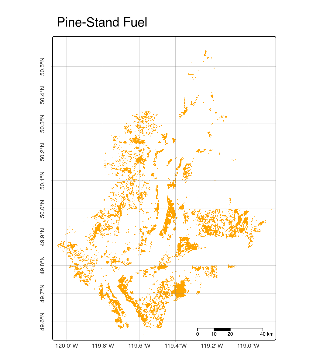
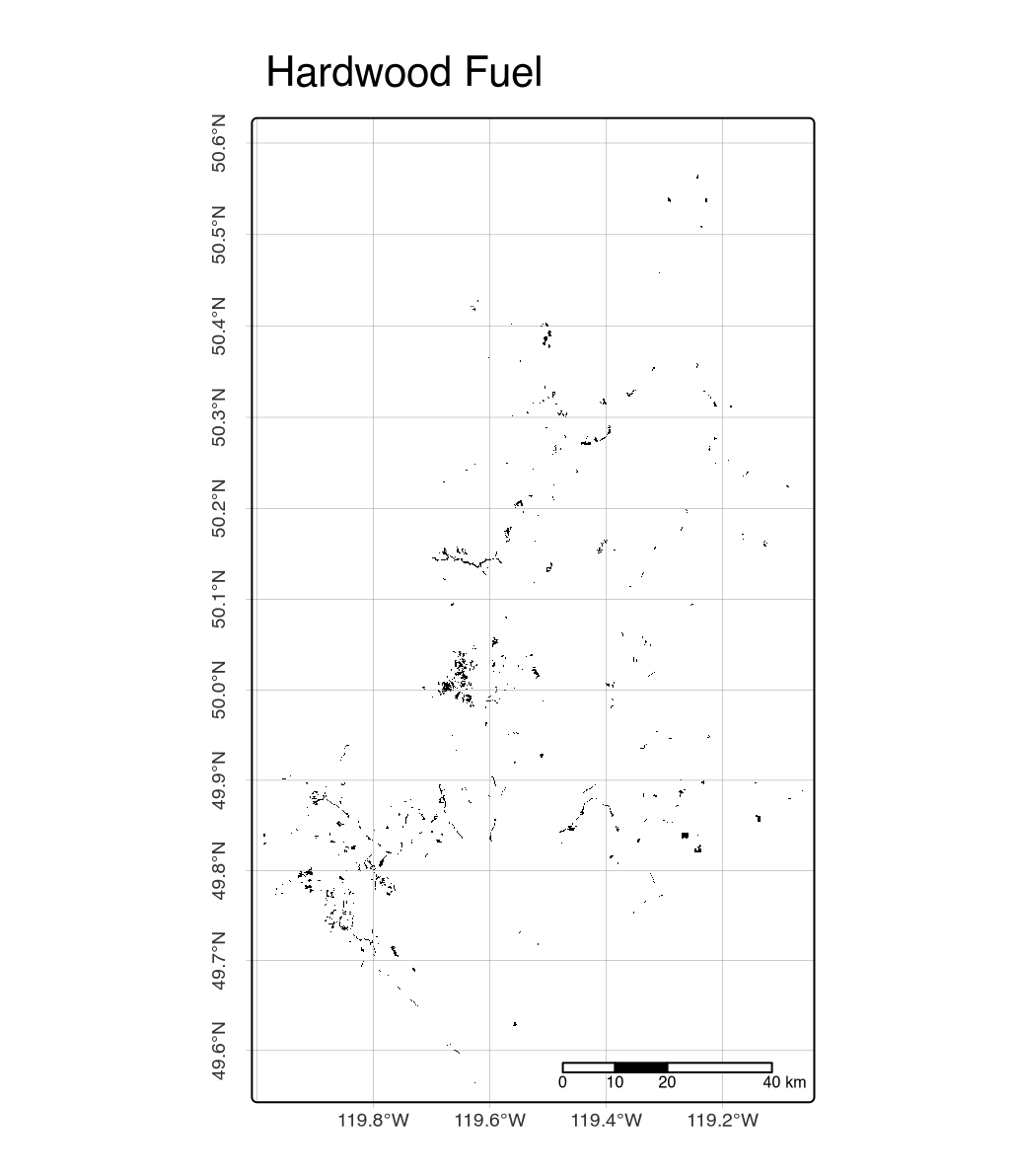
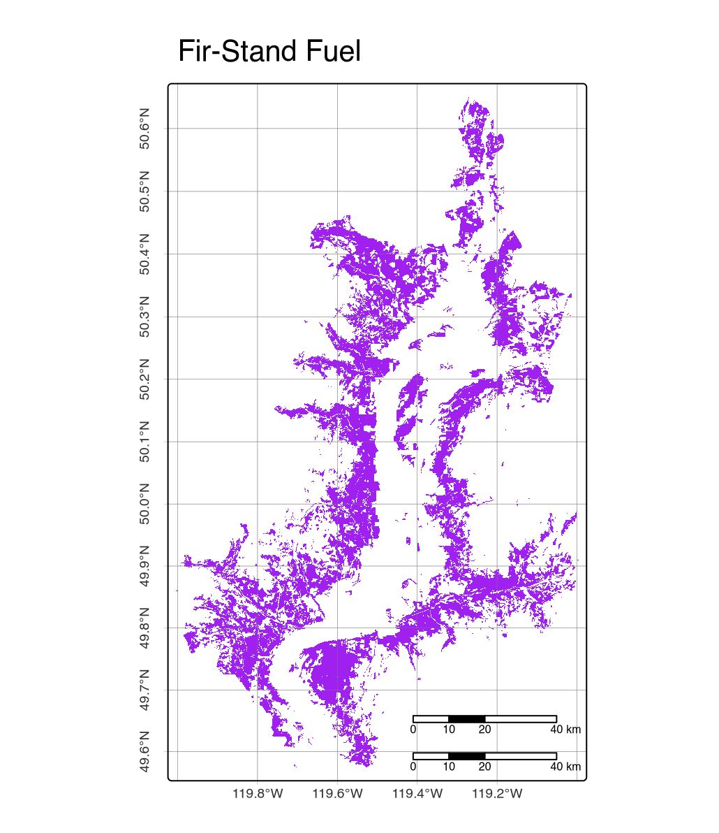
NA # ISI <int>Wotton and Beverly’s model of stand-adjusted fine fuel moisture content requires five predictor variables (Wotton and Beverly 2007). Two of these predictors were extracted from the the VRI dataset including stand type (SPEC_CD_1) and stand density (LIVE_STEMS). Rough scale criteria were used in a filtering process to classify fuel categories similar to those used in Wotton and Beverley’s model (Wotton and Beverly 2007) and more recent workflows1 (D. D. Perrakis, Eade, and Hicks 2018).
vri = st_read("./assets/VRI/vri_2022_3857.shp", quiet=T) |>
  sf::st_make_valid() |>
  dplyr::select(c(
    "BCLCS_LEVE",
    "BCLCS_LE_1",
    "BCLCS_LE_2",
    "BCLCS_LE_3",
    "BCLCS_LE_4",
    "SPECIES_CD", "SPECIES_PC",
    "BEC_ZONE_C",
    "VRI_LIVE_S"))

wotton_fuel_class = vri |>
  mutate(fuel_type = case_when((BCLCS_LEVE != "V") ~ 0,
  (BCLCS_LEVE == "V" & BCLCS_LE_3 == "TB") ~ 1,
  (BCLCS_LEVE == "V" & SPECIES_CD == "FD" | SPECIES_CD == "FDC" | SPECIES_CD == "FDI") ~ 2,
  (BCLCS_LEVE == "V" & SPECIES_PC <= 80) ~ 3,
  (BCLCS_LEVE == "V" & SPECIES_CD == "PA" | SPECIES_CD == "PL" | SPECIES_CD == "PLC" | SPECIES_CD == "PY") ~ 4,
  (BCLCS_LEVE == "V" & BCLCS_LE_4 =="SP" | SPECIES_CD == "SB" | SPECIES_CD == "SX" |
      SPECIES_CD == "SW" | SPECIES_CD == "S" | BEC_ZONE_C == "BWBS" | BEC_ZONE_C == "SWB") ~ 5, TRUE ~ 0))
Wotton_fuel_N  = dplyr::filter(vri, BCLCS_LEVE =="N")
Wotton_fuel_HW = dplyr::filter(vri, BCLCS_LE_3=="TB")
Wotton_fuel_Df = dplyr::filter(vri, BCLCS_LEVE == "V" & SPECIES_CD == "FD" | SPECIES_CD == "FDC" | SPECIES_CD == "FDI")
Wotton_fuel_MW = dplyr::filter(vri, BCLCS_LEVE == "V" & SPECIES_PC <= 80)
Wotton_fuel_PI = dplyr::filter(vri, BCLCS_LEVE == "V" & SPECIES_CD == "PA" | SPECIES_CD == "PL" | SPECIES_CD == "PLC" | SPECIES_CD == "PY")
Wotton_fuel_SP = dplyr::filter(vri, BCLCS_LEVE == "V" & BCLCS_LE_4 =="SP" | SPECIES_CD == "SB" |
    SPECIES_CD == "SX" | SPECIES_CD == "SW" | SPECIES_CD == "S" | BEC_ZONE_C == "BWBS" | BEC_ZONE_C == "SWB")

density = vri["VRI_LIVE_S"] |> dplyr::mutate(VRI_LIVE_S = as.numeric(VRI_LIVE_S))
density = rename(density, density = VRI_LIVE_S)
sf::st_write(density, "./assets/VRI/density.shp")

tmap::tm_shape(density) + tm_polygons(fill = "density",
  fill.scale = tm_scale_continuous(values = "viridis"), lwd=0,
  tm_title("Live Tree Density (Stems/ha"))
tmap::tm_shape(Wotton_fuel_N) + tm_polygons(fill = "brown", lwd=0)
tmap::tm_shape(Wotton_fuel_PI) + tm_polygons(fill = "yellow", lwd=0)
tmap::tm_shape(Wotton_fuel_HW) + tm_polygons(fill = "green", lwd=0)
tmap::tm_shape(Wotton_fuel_Df) + tm_polygons(fill = "purple", lwd=0)
tmap::tm_shape(Wotton_fuel_MW) + tm_polygons(fill = "blue", lwd=0)
tmap::tm_shape(Wotton_fuel_SP) + tm_polygons(fill = "darkgreen", lwd=0)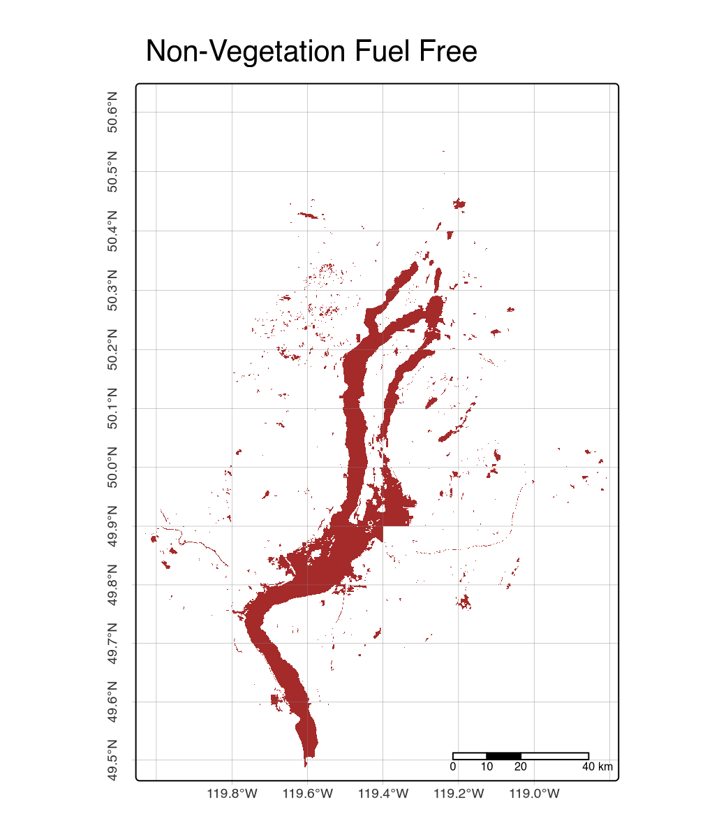 |
 |
 |
 |
 |
 |
Derive Fire Weather Maps
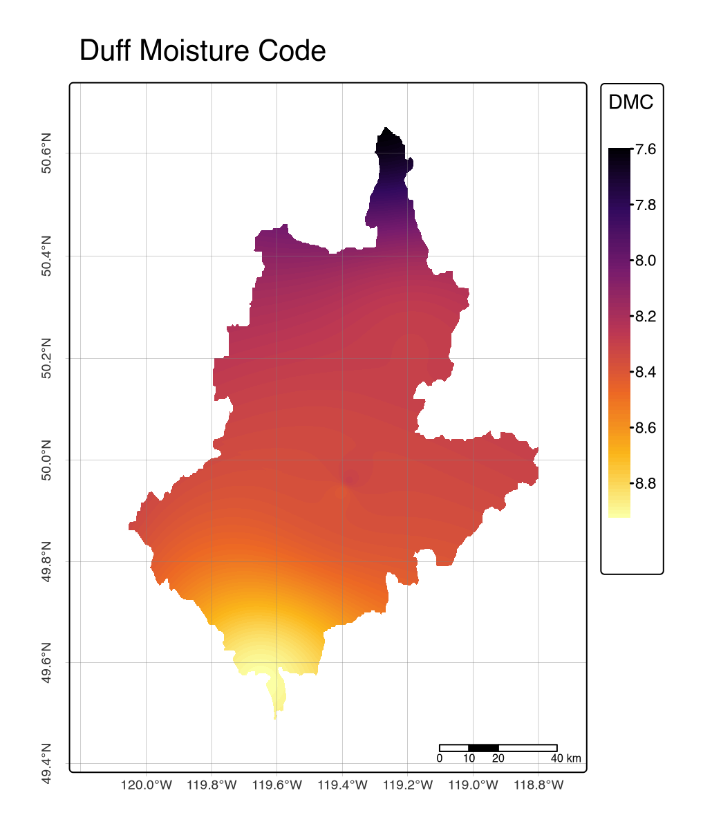
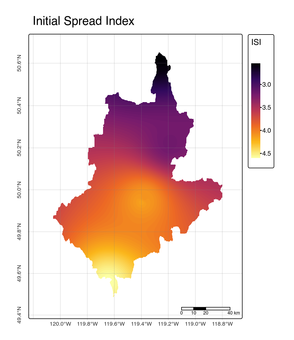
A raster stack of interpolated climate covariates was fitted to the fwiRaster function with out="all" operator. This produced raster results for Initial Spread Index (isi), and Build-up Index (bui) and other indices required in FBP calculations. This is as far as we could get and could only generate these CFFDRS outputs for generic landcover rasters; these scores need to be tuned for each fuel type area.
temp   = terra::rast("./assets/TIF/temp.tif")[[1]]
rh     = terra::rast("./assets/TIF/rh.tif")[[1]]
prec   = terra::rast("./assets/TIF/prec.tif")[[1]]
ws     = terra::rast("./assets/TIF/ws.tif")[[1]]
names(temp)   = 'temp'
names(rh)     = 'rh'
names(ws)     = 'ws'
names(prec)   = 'prec'

# Correct ordering is necessary
stack = c(temp, rh, ws, prec)

# Derive CFFDRS predictions
fwi_outputs = cffdrs::fwiRaster(stack, out = "all")

# Save as raster brick
terra::writeRaster(fwi_outputs, "./assets/TIF/fwi_outputs.tif", overwrite=T)
# Sanity check:
#names(fwi_outputs) # => "TEMP" "RH" "WS" "PREC"
#"FFMC" "DMC" "DC" "ISI" "BUI" "FWI" "DSR"
stems = sf::st_read("./assets/VRI/density.shp", quiet=T)
tmap::tmap_mode("plot")
tmap::tm_shape(fwi_outputs[["FFMC"]]) + tm_raster(style="cont", palette="inferno") +
tmap::tm_title("Fine Fuel Moisture Code") +
tmap::tm_graticules(lines=T,labels.rot=c(0,90),lwd=0.2) +
tmap::tm_scale_bar(c(0, 10, 20, 40), position = c("RIGHT", "BOTTOM"), text.size = .5)
tmap::tm_shape(fwi_outputs[["DMC"]]) + tm_raster(style="cont", palette="inferno") +
tmap::tm_title("Duff Moisture Code") +
tmap::tm_graticules(lines=T,labels.rot=c(0,90),lwd=0.2) +
tmap::tm_scale_bar(c(0, 10, 20, 40), position = c("RIGHT", "BOTTOM"), text.size = .5)
tmap::tm_shape(fwi_outputs[["DC"]]) + tm_raster(style="cont", palette="inferno") +
tmap::tm_title("Drought Code") +
tmap::tm_graticules(lines=T,labels.rot=c(0,90),lwd=0.2) +
tmap::tm_scale_bar(c(0, 10, 20, 40), position = c("RIGHT", "BOTTOM"), text.size = .5)
tmap::tm_shape(fwi_outputs[["ISI"]]) + tm_raster(style="cont", palette="inferno") +
tmap::tm_title("Initial Spread Index") +
tmap::tm_graticules(lines=T,labels.rot=c(0,90),lwd=0.2) +
tmap::tm_scale_bar(c(0, 10, 20, 40), position = c("RIGHT", "BOTTOM"), text.size = .5)
tmap::tm_shape(fwi_outputs[["BUI"]]) + tm_raster(style="cont", palette="inferno") +
tmap::tm_title("Buildup Index") +
tmap::tm_graticules(lines=T,labels.rot=c(0,90),lwd=0.2) +
tmap::tm_scale_bar(c(0, 10, 20, 40), position = c("RIGHT", "BOTTOM"), text.size = .5)
tmap::tm_shape(fwi_outputs[["FWI"]]) + tm_raster(style="cont", palette="inferno") +
tmap::tm_title("Fire Weather Index") +
tmap::tm_graticules(lines=T,labels.rot=c(0,90),lwd=0.2) +
tmap::tm_scale_bar(c(0, 10, 20, 40), position = c("RIGHT", "BOTTOM"), text.size = .5)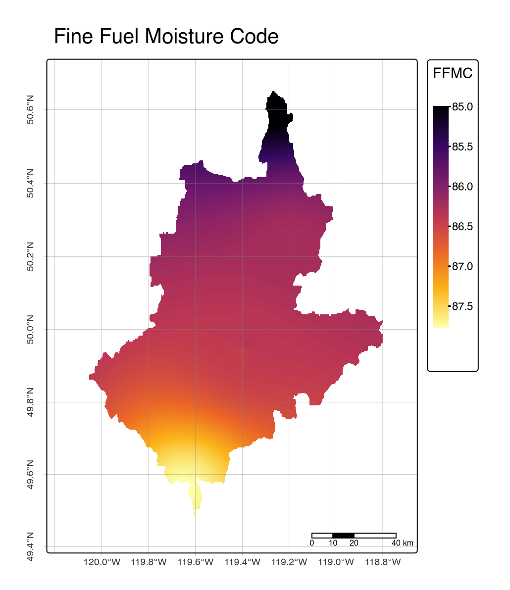 |
 |
 |
 |
 |
 |
Daily Fire Severity |
 |

Derive Fire Prediction Maps
Derive Fire Prediction Maps
With the necessary fire weather and fuel type data prepared, the final step involves applying a stand-adjusted fine-fuel moisture content model. The following values adopted from published study by Perrakis and others (D. D. B. Perrakis et al. 2014) looking effects of beetle-induced tree mortality on forest fuels and fire behaviour within pine stands the southern interior of British Columbia. The core samc function takes the weather-based FFMC and DMC indices and adjusts them according to previously derived stand-specific predictors, including stand type and density. This final calculation provides a critical link between general climate-driven fire danger ratings and localized fire behavior predictions that account for on-the-ground forest characteristics.
#define mcF, mcD, ex.mod intermediate functions
mcF    = function(ffmc){147.2*(101-ffmc)/(59.5+ffmc)}
mcD    = function(dmc) {20+exp(-(dmc-244.72)/43.43)}
ex.mod = function(s1, s2, s3, ffmc, dmc) {exp(s1+s2*log(mcF(ffmc))+s3*mcD(dmc))}

#define stand-adjusted mc function to build FFMC, DMC, stand, density, season
samc<-function(ffmc, dmc, stand, density, season) {
  #Get coefficients
  CoTr1 <-c(
    0.7299,0.0202,0.7977,0.8517,0.7391,
    0.4387,-0.271,0.5065,0.5605,0.4479,
    -0.2449,-0.9546,-0.1771,-0.1231,-0.2357,
    0.1348,-0.5749,0.2026,0.2566,0.144,
    -0.1564,-0.8661,-0.0886,-0.0346,-0.1472,
    -0.84,-1.5497,-0.7722,-0.7182,-0.8308,
    0.1601,-0.55,0.2279,0.2819,0.1693,
    -0.1311,-0.8408,-0.0633,-0.0093,-0.1219,
    -0.8147,-1.5244,-0.7469,-0.6929,-0.8055)
  CoTr2 <- c(
    0.5221,0.6264,0.5042,0.3709,0.4285,
    0.7133,0.8176,0.6954,0.5621,0.6197,
    1.0462,1.1505,1.0283,0.895,0.9526,
    0.8691,0.9734,0.8512,0.7179,0.7755,
    1.0603,1.1646,1.0424,0.9091,0.9667,
    1.3932,1.4975,1.3753,1.242,1.2996,
    0.9495,1.0538,0.9316,0.7983,0.8559,
    1.1407,1.245,1.1228,0.9895,1.0471,
    1.4736,1.5779,1.4557,1.3224,1.38)
  co3 <- 0.002232

  #Create data frame for pulling coefs
  AllCo <-data.frame("co1"=CoTr1, "co2"=CoTr2)

  #Spring and Summer coefs for 'sprummer' model
  co_sp <- AllCo[1:15,]
  co_su <- AllCo[16:30,]


  if(season==1.5) {
    #spring
    c1.sprD=co_sp[(density*5-4):(density*5), 1]
    c2.sprD=co_sp[(density*5-4):(density*5), 2]
    c1=c1.sprD[stand]
    c2=c2.sprD[stand]
    mc.spr=ex.mod(c1, c2, co3, ffmc, dmc)
    #summer
    c1.sumD=co_su[(density*5-4):(density*5), 1]
    c2.sumD=co_su[(density*5-4):(density*5), 2]
    c3=c1.sumD[stand]
    c4=c2.sumD[stand]
    mc.sum=ex.mod(c3, c4, co3, ffmc, dmc)

    #final 'sprummer' mc calc
    return(mean(c(mc.spr, mc.sum)))

    #for all others - spring, summer or fall
  } else {
    c1a=AllCo$co1[(season*15-14):(season*15)]
    c2a=AllCo$co2[(season*15-14):(season*15)]
    c1b=c1a[(density*5-4):(density*5)]
    c2b=c2a[(density*5-4):(density*5)]
    c1c=c1b[stand]
    c2c=c2b[stand]
    return(ex.mod(c1c, c2c, co3, ffmc, dmc))
  }
}
Runtime log
devtools::session_info()─ Session info ──────────────────────────────────────────────────
setting value
version R version 4.3.0 (2023-04-21)
os macOS 15.6.1
system aarch64, darwin20
ui RStudio
language (EN)
collate en_US.UTF-8
ctype en_US.UTF-8
tz America/Vancouver
date 2025-09-01
rstudio 2024.12.1+563 Kousa Dogwood (desktop)
pandoc 3.6.1 @ /usr/local/bin/ (via rmarkdown)
quarto 1.7.33 @ /usr/local/bin/quarto
─ Packages ──────────────────────────────────────────────────────
! package * version date (UTC) lib source
P abind 1.4-8 2024-09-12 [?] CRAN (R 4.3.3)
P backports 1.5.0 2024-05-23 [?] CRAN (R 4.3.3)
P base64enc 0.1-3 2015-07-28 [?] CRAN (R 4.3.3)
P bibtex * 0.5.1 2023-01-26 [?] CRAN (R 4.3.3)
P brew 1.0-10 2023-12-16 [?] CRAN (R 4.3.3)
P bslib 0.9.0 2025-01-30 [?] CRAN (R 4.3.3)
P cachem 1.1.0 2024-05-16 [?] CRAN (R 4.3.3)
P cartogram 0.3.0 2023-05-26 [?] CRAN (R 4.3.0)
P cffdrs * 1.9.2 2025-08-22 [?] CRAN (R 4.3.0)
P chromote * 0.5.1 2025-04-24 [?] CRAN (R 4.3.3)
P class 7.3-23 2025-01-01 [?] CRAN (R 4.3.3)
P classInt 0.4-11 2025-01-08 [?] CRAN (R 4.3.3)
P cli 3.6.5 2025-04-23 [?] CRAN (R 4.3.3)
P codetools 0.2-20 2024-03-31 [?] CRAN (R 4.3.1)
P colorspace 2.1-1 2024-07-26 [?] CRAN (R 4.3.3)
P cols4all * 0.9 2025-08-28 [?] CRAN (R 4.3.0)
P coro 1.1.0 2024-11-05 [?] CRAN (R 4.3.3)
P crosstalk 1.2.2 2025-08-26 [?] CRAN (R 4.3.0)
P curl * 7.0.0 2025-08-19 [?] CRAN (R 4.3.0)
P data.table 1.17.8 2025-07-10 [?] CRAN (R 4.3.3)
P DBI 1.2.3 2024-06-02 [?] CRAN (R 4.3.3)
P deldir 2.0-4 2024-02-28 [?] CRAN (R 4.3.3)
P devtools * 2.4.5 2022-10-11 [?] CRAN (R 4.3.0)
P dichromat 2.0-0.1 2022-05-02 [?] CRAN (R 4.3.3)
P digest 0.6.37 2024-08-19 [?] CRAN (R 4.3.3)
P doParallel 1.0.17 2022-02-07 [?] CRAN (R 4.3.3)
P dplyr * 1.1.4 2023-11-17 [?] CRAN (R 4.3.1)
P e1071 1.7-16 2024-09-16 [?] CRAN (R 4.3.3)
P elevatr * 0.99.0 2023-09-12 [?] CRAN (R 4.3.0)
P ellipsis 0.3.2 2021-04-29 [?] CRAN (R 4.3.3)
P ellmer * 0.3.1 2025-08-24 [?] CRAN (R 4.3.0)
P evaluate 1.0.5 2025-08-27 [?] CRAN (R 4.3.0)
P farver 2.1.2 2024-05-13 [?] CRAN (R 4.3.3)
P fastmap 1.2.0 2024-05-15 [?] CRAN (R 4.3.3)
P FNN 1.1.4.1 2024-09-22 [?] CRAN (R 4.3.3)
P foreach 1.5.2 2022-02-02 [?] CRAN (R 4.3.3)
P fs 1.6.6 2025-04-12 [?] CRAN (R 4.3.3)
P generics 0.1.4 2025-05-09 [?] CRAN (R 4.3.3)
P geonetwork * 0.6.0 2025-07-23 [?] CRAN (R 4.3.0)
P ggplot2 * 3.5.2 2025-04-09 [?] CRAN (R 4.3.3)
P glue 1.8.0 2024-09-30 [?] CRAN (R 4.3.3)
P gstat * 2.1-4 2025-07-10 [?] CRAN (R 4.3.3)
P gtable 0.3.6 2024-10-25 [?] CRAN (R 4.3.3)
P hexbin 1.28.5 2024-11-13 [?] CRAN (R 4.3.3)
P htmltools * 0.5.8.1 2024-04-04 [?] CRAN (R 4.3.3)
P htmlwidgets 1.6.4 2023-12-06 [?] CRAN (R 4.3.1)
P httpuv 1.6.16 2025-04-16 [?] CRAN (R 4.3.3)
P httr2 * 1.2.1 2025-07-22 [?] CRAN (R 4.3.0)
P igraph 2.1.4 2025-01-23 [?] CRAN (R 4.3.3)
P interp 1.1-6 2024-01-26 [?] CRAN (R 4.3.3)
P intervals 0.15.5 2024-08-23 [?] CRAN (R 4.3.3)
P iterators 1.0.14 2022-02-05 [?] CRAN (R 4.3.3)
P janitor * 2.2.1 2024-12-22 [?] CRAN (R 4.3.3)
P jpeg 0.1-11 2025-03-21 [?] CRAN (R 4.3.3)
P jquerylib 0.1.4 2021-04-26 [?] CRAN (R 4.3.3)
P jsonlite 2.0.0 2025-03-27 [?] CRAN (R 4.3.3)
P kableExtra * 1.4.0 2024-01-24 [?] CRAN (R 4.3.1)
P KernSmooth 2.23-26 2025-01-01 [?] CRAN (R 4.3.3)
P knitr * 1.50 2025-03-16 [?] CRAN (R 4.3.3)
P later 1.4.4 2025-08-27 [?] CRAN (R 4.3.0)
P lattice * 0.22-7 2025-04-02 [?] CRAN (R 4.3.3)
P latticeExtra 0.6-30 2022-07-04 [?] CRAN (R 4.3.3)
P leafem 0.2.5 2025-08-28 [?] CRAN (R 4.3.0)
P leaflegend 1.2.1 2024-05-09 [?] CRAN (R 4.3.3)
P leaflet 2.2.2 2024-03-26 [?] CRAN (R 4.3.1)
P leaflet.providers 2.0.0 2023-10-17 [?] CRAN (R 4.3.3)
P leafpop 0.1.0 2021-05-22 [?] CRAN (R 4.3.0)
P leafsync 0.1.0 2019-03-05 [?] CRAN (R 4.3.0)
P lifecycle 1.0.4 2023-11-07 [?] CRAN (R 4.3.3)
P logger 0.4.0 2024-10-22 [?] CRAN (R 4.3.3)
P lubridate 1.9.4 2024-12-08 [?] CRAN (R 4.3.3)
P lutz * 0.3.2 2023-10-17 [?] CRAN (R 4.3.3)
P lwgeom 0.2-14 2024-02-21 [?] CRAN (R 4.3.1)
P magrittr 2.0.3 2022-03-30 [?] CRAN (R 4.3.3)
P mapedit * 0.7.0 2025-04-20 [?] CRAN (R 4.3.3)
P maptiles 0.10.0 2025-05-07 [?] CRAN (R 4.3.3)
P mapview 2.11.3 2025-08-28 [?] CRAN (R 4.3.0)
P memoise 2.0.1 2021-11-26 [?] CRAN (R 4.3.3)
P mime 0.13 2025-03-17 [?] CRAN (R 4.3.3)
P miniUI 0.1.2 2025-04-17 [?] CRAN (R 4.3.3)
P ncdf4 * 1.24 2025-03-25 [?] CRAN (R 4.3.3)
P OpenStreetMap * 0.4.0 2023-10-12 [?] CRAN (R 4.3.1)
P openxlsx * 4.2.8 2025-01-25 [?] CRAN (R 4.3.3)
P osmdata * 0.3.0 2025-08-23 [?] CRAN (R 4.3.0)
P packcircles 0.3.7 2024-11-21 [?] CRAN (R 4.3.3)
P pacman 0.5.1 2019-03-11 [?] CRAN (R 4.3.3)
pandoc * 0.2.0 2023-08-24 [1] CRAN (R 4.3.3)
P pandocfilters * 0.1-6 2022-08-11 [?] CRAN (R 4.3.3)
P pillar 1.11.0 2025-07-04 [?] CRAN (R 4.3.3)
P pkgbuild 1.4.8 2025-05-26 [?] CRAN (R 4.3.3)
P pkgconfig 2.0.3 2019-09-22 [?] CRAN (R 4.3.3)
P pkgload 1.4.0 2024-06-28 [?] CRAN (R 4.3.3)
P plyr 1.8.9 2023-10-02 [?] CRAN (R 4.3.3)
P png 0.1-8 2022-11-29 [?] CRAN (R 4.3.3)
P processx 3.8.6 2025-02-21 [?] CRAN (R 4.3.3)
P profvis 0.4.0 2024-09-20 [?] CRAN (R 4.3.3)
P progressr 0.15.1 2024-11-22 [?] CRAN (R 4.3.3)
P PROJ * 0.6.0 2025-04-03 [?] CRAN (R 4.3.3)
P proj4 1.0-15 2025-03-21 [?] CRAN (R 4.3.3)
P promises 1.3.3 2025-05-29 [?] CRAN (R 4.3.3)
P proxy 0.4-27 2022-06-09 [?] CRAN (R 4.3.3)
P ps 1.9.1 2025-04-12 [?] CRAN (R 4.3.3)
P purrr 1.1.0 2025-07-10 [?] CRAN (R 4.3.0)
P R6 2.6.1 2025-02-15 [?] CRAN (R 4.3.3)
P rappdirs 0.3.3 2021-01-31 [?] CRAN (R 4.3.3)
P raster * 3.6-32 2025-03-28 [?] CRAN (R 4.3.3)
P rasterVis * 0.51.6 2023-11-01 [?] CRAN (R 4.3.3)
P RColorBrewer 1.1-3 2022-04-03 [?] CRAN (R 4.3.3)
P Rcpp 1.1.0 2025-07-02 [?] CRAN (R 4.3.3)
P remotes 2.5.0 2024-03-17 [?] CRAN (R 4.3.3)
renv * 1.1.5 2025-07-24 [1] CRAN (R 4.3.0)
P reproj * 0.7.0 2024-06-11 [?] CRAN (R 4.3.3)
P rJava 1.0-11 2024-01-26 [?] CRAN (R 4.3.3)
P rlang 1.1.6 2025-04-11 [?] CRAN (R 4.3.3)
P rmapshaper * 0.5.0 2023-04-11 [?] CRAN (R 4.3.0)
P rmarkdown * 2.29 2024-11-04 [?] CRAN (R 4.3.3)
P rstudioapi 0.17.1 2024-10-22 [?] CRAN (R 4.3.3)
P s2 1.1.9 2025-05-23 [?] CRAN (R 4.3.3)
P S7 0.2.0 2024-11-07 [?] CRAN (R 4.3.3)
P sass 0.4.10 2025-04-11 [?] CRAN (R 4.3.3)
P satellite 1.0.6 2025-08-21 [?] CRAN (R 4.3.0)
P scales 1.4.0 2025-04-24 [?] CRAN (R 4.3.3)
P sessioninfo 1.2.3 2025-02-05 [?] CRAN (R 4.3.3)
P sf * 1.0-22 2025-08-25 [?] Github (r-spatial/sf@3660edf)
P shiny 1.11.1 2025-07-03 [?] CRAN (R 4.3.3)
P shinyWidgets 0.9.0 2025-02-21 [?] CRAN (R 4.3.3)
P snakecase 0.11.1 2023-08-27 [?] CRAN (R 4.3.0)
P sp * 2.2-0 2025-02-01 [?] CRAN (R 4.3.3)
P spacesXYZ 1.6-0 2025-06-06 [?] CRAN (R 4.3.3)
P spacetime 1.3-3 2025-02-13 [?] CRAN (R 4.3.3)
P stars 0.6-8 2025-02-01 [?] CRAN (R 4.3.3)
P stringi 1.8.7 2025-03-27 [?] CRAN (R 4.3.3)
P stringr 1.5.1 2023-11-14 [?] CRAN (R 4.3.1)
P svglite 2.2.1 2025-05-12 [?] CRAN (R 4.3.3)
P systemfonts 1.2.3 2025-04-30 [?] CRAN (R 4.3.3)
P terra * 1.8-60 2025-07-21 [?] CRAN (R 4.3.0)
P textshaping 1.0.1 2025-05-01 [?] CRAN (R 4.3.3)
P tibble 3.3.0 2025-06-08 [?] CRAN (R 4.3.3)
P tidyselect 1.2.1 2024-03-11 [?] CRAN (R 4.3.1)
P timechange 0.3.0 2024-01-18 [?] CRAN (R 4.3.3)
P tinytex * 0.57 2025-04-15 [?] CRAN (R 4.3.3)
tmap * 4.1 2025-05-12 [1] CRAN (R 4.3.3)
tmap.cartogram * 0.2 2025-05-14 [1] CRAN (R 4.3.3)
tmap.glyphs * 0.1 2025-05-30 [1] CRAN (R 4.3.3)
tmap.networks * 0.1 2025-05-30 [1] CRAN (R 4.3.3)
P tmaptools * 3.2 2025-01-13 [?] CRAN (R 4.3.3)
P units 0.8-7 2025-03-11 [?] CRAN (R 4.3.3)
P urlchecker 1.0.1 2021-11-30 [?] CRAN (R 4.3.3)
P useful * 1.2.6.1 2023-10-24 [?] CRAN (R 4.3.1)
P usethis * 3.2.0 2025-08-28 [?] CRAN (R 4.3.0)
P uuid 1.2-1 2024-07-29 [?] CRAN (R 4.3.3)
P V8 6.0.6 2025-08-18 [?] CRAN (R 4.3.0)
P vctrs 0.6.5 2023-12-01 [?] CRAN (R 4.3.3)
P viridisLite 0.4.2 2023-05-02 [?] CRAN (R 4.3.3)
P weathercan * 0.7.5 2025-08-26 [?] https://ropensci.r-universe.dev (R 4.3.0)
P websocket 1.4.4 2025-04-10 [?] CRAN (R 4.3.3)
P withr 3.0.2 2024-10-28 [?] CRAN (R 4.3.3)
P wk 0.9.4 2024-10-11 [?] CRAN (R 4.3.3)
P xfun 0.53 2025-08-19 [?] CRAN (R 4.3.0)
P XML 3.99-0.18 2025-01-01 [?] CRAN (R 4.3.3)
P xml2 1.4.0 2025-08-20 [?] CRAN (R 4.3.0)
P xtable 1.8-4 2019-04-21 [?] CRAN (R 4.3.3)
P xts 0.14.1 2024-10-15 [?] CRAN (R 4.3.3)
P yaml 2.3.10 2024-07-26 [?] CRAN (R 4.3.3)
P zip 2.3.3 2025-05-13 [?] CRAN (R 4.3.3)
P zoo 1.8-14 2025-04-10 [?] CRAN (R 4.3.3)
[1] /Users/seamus/repos/forest-fire-risk-cffdrs/renv/library/R-4.3/aarch64-apple-darwin20
[2] /Users/seamus/Library/Caches/org.R-project.R/R/renv/sandbox/R-4.3/aarch64-apple-darwin20/ac5c2659
* ── Packages attached to the search path.
P ── Loaded and on-disk path mismatch.
─────────────────────────────────────────────────────────────────References
Boucher, J, C Hanes, N Jurko, D Perrais, S Taylor, D Thompson, and M Wottom. n.d. “The Vision for the Next Generation of the Canadian Forest Fire Danger Rating System.”
Hollister, Jeffrey, Tarak Shah, Jakub Nowosad, Alec L. Robitaille, Marcus W. Beck, and Mike Johnson. 2023. “Elevatr: Access Elevation Data from Various APIs.” https://doi.org/10.5281/zenodo.8335450.
Perrakis, Daniel D. B., Rick A. Lanoville, Stephen W. Taylor, and Dana Hicks. 2014. “Modeling Wildfire Spread in Mountain Pine Beetle-Affected Forest Stands, British Columbia, Canada.” Fire Ecology 10 (2): 10–35. https://doi.org/10.4996/fireecology.1002010.
Perrakis, Daniel DB, Miguel G Cruz, Martin E Alexander, Chelene C Hanes, Dan K Thompson, Stephen W Taylor, and Brian J Stocks. 2023. “Improved Logistic Models of Crown Fire Probability in Canadian Conifer Forests.” International Journal of Wildland Fire 32 (10): 14551473.
Perrakis, Daniel DB, George Eade, and Dana Hicks. 2018. “British Columbia Wildfire Fuel Typing and Fuel Type Layer Description.”
Wotton, B Mike, and Jennifer L Beverly. 2007. “Stand-Specific Litter Moisture Content Calibrations for the Canadian Fine Fuel Moisture Code.” International Journal of Wildland Fire 16 (4): 463472.
Footnotes
Additional fuel typing layers available in VRI datasets that are yet under-explored/lacking research: SHRB_HT, SHRB_CC, HERB_TYPE, HERB_COVER, HERB_PCT, NON_VEG_1, N_LOG_DATE, DEAD_PCT, HRVSTDT, SITE_INDEX, PROJ_HT_1, #SPEC_AGE_1, DEAD_PCT, STEM_HA_CD, DEAD_STEMS, NVEG_COV_1)↩︎